Tail Risk

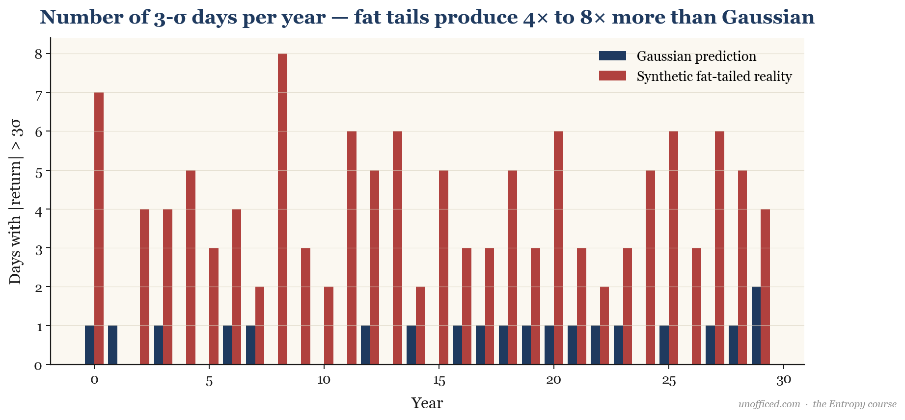
In financial markets, ‘risk’ often refers to the predictable ups and downs, the volatility we can measure with standard deviation. But there’s a more dangerous kind of risk lurking in the shadows: tail risk. This is the risk of an event so far outside the norm that it can wipe out weeks or months of gains in a single session. While statistical theory based on the normal distribution (the bell curve) treats these events as once-in-a-lifetime occurrences, the reality in Indian markets is that they happen far more frequently. Understanding this mismatch is critical for survival. The infamous 1998 collapse of Long-Term Capital Management (LTCM) serves as the quintessential cautionary tale, where a portfolio of supposedly uncorrelated trades simultaneously imploded in what their Gaussian models deemed a ten-sigma event—an impossibility in theory, a catastrophe in practice.

Value at Risk (VaR)

Value at Risk, or VaR, is a standard metric used to quantify the level of financial risk within a firm or portfolio over a specific time frame. For a given portfolio, time horizon, and probability , the VaR is the threshold loss value such that the probability that the loss on the portfolio over the given time horizon exceeds this value is .

Mathematically, for a random variable representing profit and loss (where loss is negative), the VaR at confidence level is the negative of the -quantile of the distribution:

Where is the cumulative distribution function of . A 99% VaR, for example, uses .

Under the simplifying assumption of a normal distribution with mean and standard deviation , the VaR can be calculated directly:

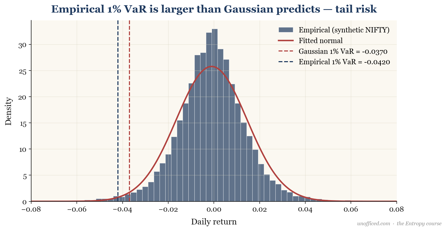
Where is the inverse of the standard normal CDF. For a 1% VaR (), . If we assume a mean daily return of zero, the 1% VaR is simply .

However, empirical data from Indian indices like NIFTY tells a different story. When we measure the actual 1% VaR from historical returns, we find it is consistently larger than this theoretical value. It is common for the empirical 1% VaR to be 1.4 to 1.8 times the size of the Gaussian VaR. This means a “one-in-a-hundred day” loss is both more frequent and more severe than the textbook model predicts.

Expected Shortfall (ES)

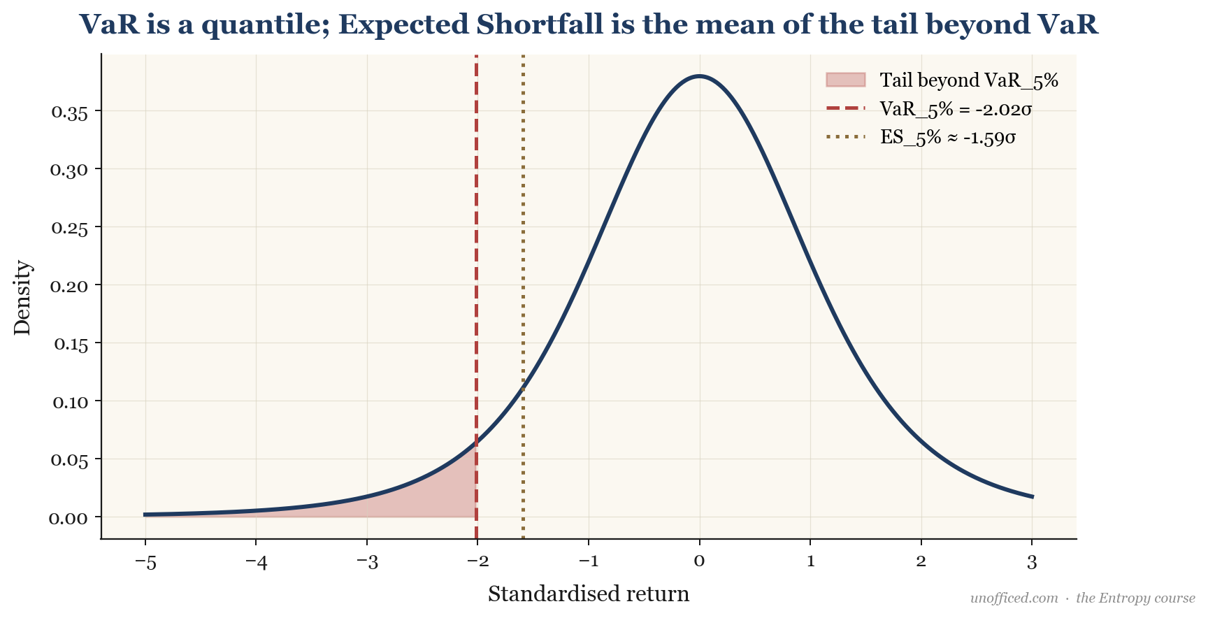
While VaR tells us the maximum loss we don’t expect to exceed, it doesn’t tell us what happens if we *do* exceed it. That’s where Expected Shortfall (ES), also known as Conditional VaR (CVaR), comes in. It answers the crucial question: “If things go badly (i.e., we breach the VaR threshold), how bad do we expect them to be?” It’s the expected loss *given* that the loss is greater than or equal to the VaR.

The formula is the average of all losses in the tail beyond the VaR quantile:

For a normal distribution, the ES also has a convenient formula:

Where is the standard normal probability density function (PDF). For a 1% ES () and assuming , this simplifies to approximately . ES is considered a “coherent” risk measure, while VaR is not, because it better captures the properties of diversification.

Extreme Value Theory (EVT)

VaR and ES calculations based on the normal distribution fail precisely because they use a model that doesn’t fit the most important data points—the extremes. Extreme Value Theory (EVT) offers a more robust framework by focusing specifically on the behaviour of tails, without making strong assumptions about the overall distribution.

There are two primary methods in EVT:

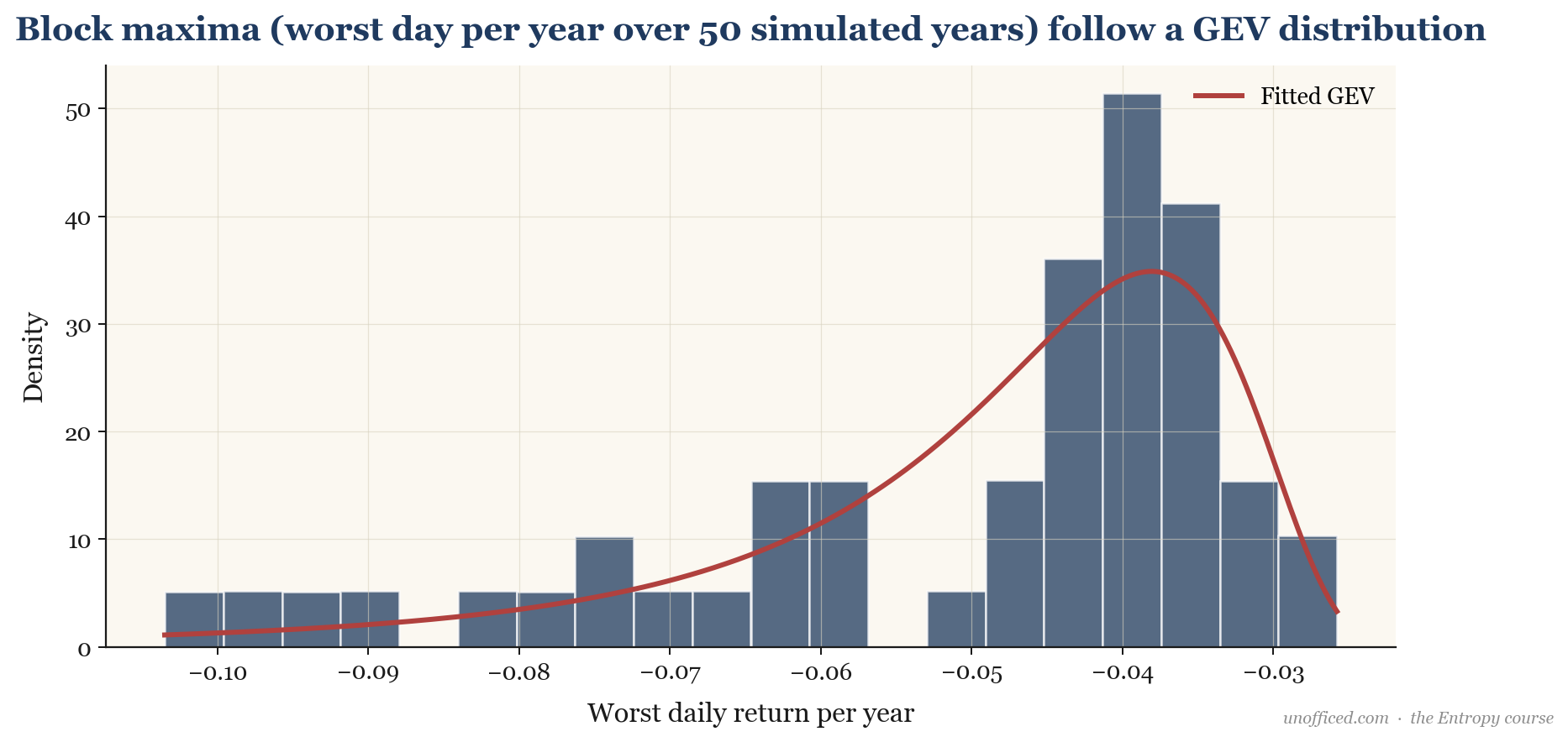
1. Block Maxima (GEV Distribution)

In this approach, the data is divided into non-overlapping blocks of equal size (e.g., the worst daily loss each month). The Fisher–Tippett–Gnedenko theorem, a cornerstone of EVT, states that the distribution of these block maxima (or minima) can only converge to one of three types, which are unified in the Generalised Extreme Value (GEV) distribution.

The most important parameter here is , the shape parameter, which determines the tail behaviour. For financial returns, we consistently find , corresponding to a heavy-tailed Fréchet distribution.

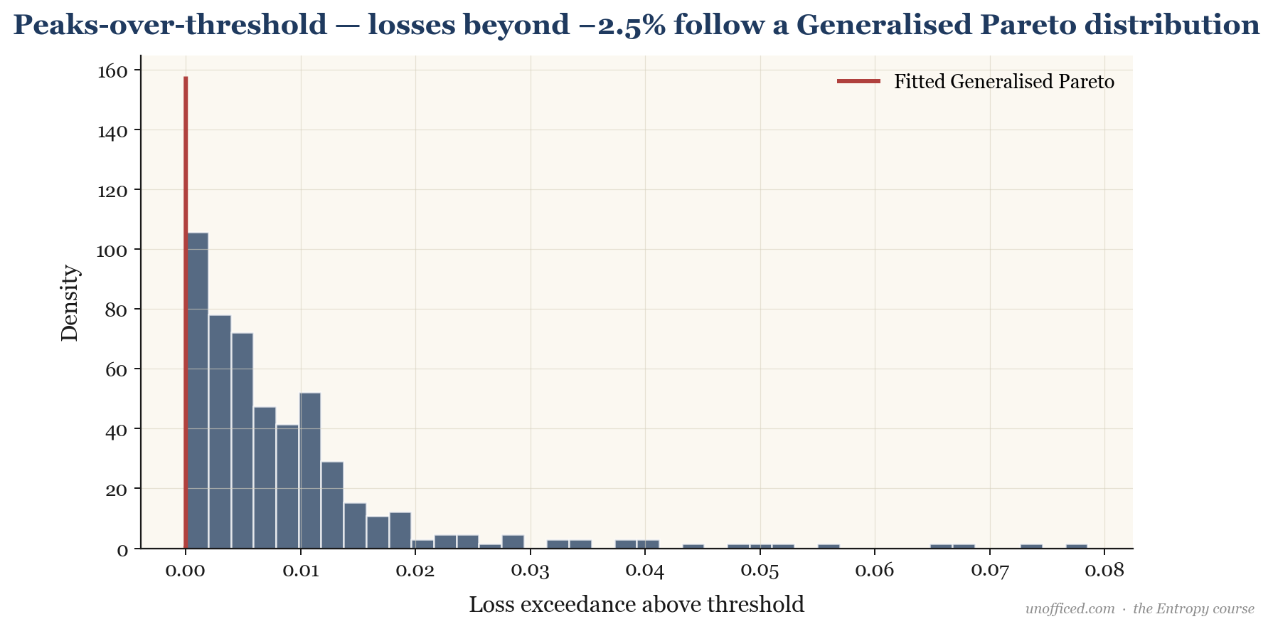
2. Peaks-Over-Threshold (GPD)

A more data-efficient method is to choose a high threshold (e.g., all daily losses greater than 2%) and model the distribution of the excesses beyond this threshold. The Pickands-Balkema-de Haan theorem states that for a large class of distributions, these excesses will follow a Generalised Pareto Distribution (GPD).

Again, the shape parameter is the signature of a heavy-tailed process, and this is what we find when we apply this method to NIFTY and BankNifty returns.

Sources of Tail Risk in Indian Markets

The “fat tails” in Indian market returns aren’t just a statistical quirk; they are driven by specific, recurring market phenomena.

• Earnings-day Gaps: Individual stocks can experience massive overnight gaps (up or down) of 10-20% following the release of quarterly earnings reports, especially if they contain a surprise. A position sized for a 2% daily volatility can be catastrophic in this environment.
• BankNifty Overnight Gaps: As a volatile, news-sensitive index, BankNifty is prone to large overnight gaps following global cues, RBI policy announcements, or sector-specific news. With a lot size of 15 and a tick value of Rs. 0.05, even a seemingly small 200-point gap can have a significant P/L impact on an F&O position.
• SEBI Circuit-Breaker Events: Both individual stocks and indices are subject to circuit limits (e.g., 10%, 15%, 20% for indices). While designed to curb panic, hitting a circuit breaker is by definition a tail event and often leads to locked limits with no exit for traders on the wrong side.
• Black Swan Macro Events: Unforeseeable events can have a cascading effect. The Adani-Hindenburg episode in January 2023 is a prime example, where allegations against a single conglomerate led to multiple days of multi-sigma moves in its constituent stocks, dragging down the broader indices with them.

Implications for Bollinger Band Trading

The fact that returns are not normally distributed has direct consequences for any strategy based on standard deviations, such as Bollinger Bands.

Defence: Sizing, Stress-Testing, and Humility

The most important defences against tail risk are operational, not just statistical.

1. Position Sizing

The single most important defence is disciplined position sizing. A common rule of thumb for robust trading systems is to risk no more than 1% of your total account equity on any single trade. The mathematical justification for this lies in the nature of recovery from drawdowns. Under a fat-tailed distribution, the probability of a string of large losses is higher than under a normal one. The path to recover from a deep drawdown is convex—it requires disproportionately larger percentage gains to get back to breakeven. An even more robust rule for a trader:

Never size a position such that a 5-sigma event (which we know happens more often than theory suggests) can ruin your account.

2. Stress Testing

Stress testing involves asking “what if” questions to understand portfolio vulnerabilities. This isn’t a statistical exercise but a scenario-based one. For example: “What happens to my F&O portfolio if NIFTY gaps down 4% overnight and VIX doubles from 12 to 24?” This forces a trader to confront the combined effects of delta and vega risk in a crisis scenario, something a simple VaR calculation will miss.

Summary

To navigate the markets effectively, we must trade the market we have, not the one from the textbooks.

• Tail risk refers to the greater-than-expected frequency and magnitude of large losses, a phenomenon mathematically described as “fat tails” or leptokurtosis.
• Empirical VaR and Expected Shortfall in Indian markets are significantly higher than theoretical Gaussian values, rendering normal distribution models dangerous for risk management.
• Extreme Value Theory (EVT) provides a more accurate framework for modelling the tails by using distributions like GEV and GPD, which mathematically confirm the heavy-tailed nature of returns.
• Key drivers of tail risk include earnings gaps, BankNifty behaviour, and black swan events.
• Standard deviation-based indicators like Bollinger Bands are less reliable than theory suggests; touches and breaches are more common.
• The most crucial defences against tail risk are operational: strict position sizing (e.g., the 1% rule), scenario-based stress testing, and a healthy respect for the market’s capacity for extreme moves.

With this understanding of the market’s true distributional properties, we can now build a more robust framework for using indicators like Bollinger Bands for generating trade setups.

Further Reading

1. “Options, Futures, and Other Derivatives” by John C. Hull: The definitive textbook introduction to the mechanics of VaR and Expected Shortfall.
2. “Modelling of Extremal Events for Insurance and Finance” by Paul Embrechts, Claudia Klüppelberg, and Thomas Mikosch: The academic bible for Extreme Value Theory. A dense but comprehensive reference.
3. “The Black Swan: The Impact of the Highly Improbable” by Nassim Nicholas Taleb: A philosophical and highly readable exploration of the importance of tail events and the intellectual fraud of relying on Gaussian models in finance.
4. “Measuring Market Risk” by Kevin Dowd: A practical, hands-on guide to the implementation and limitations of various market risk models.