Kurtosis

What is Kurtosis?
Kurtosis is a statistical measure that quantifies the “tailedness” of a probability distribution. Unlike variance, which measures the magnitude of typical deviations from the mean, kurtosis measures the frequency and magnitude of extreme deviations—the “outliers.” A distribution with high kurtosis is said to have “heavy tails” or “fat tails,” meaning that extreme outcomes occur far more frequently than a normal (Gaussian) distribution would predict.
In trading and quantitative finance, kurtosis is a direct measure of tail risk. It tells us how often we can expect market returns to experience massive, multi-standard-deviation moves. Financial returns are famously not normal, and kurtosis provides a precise way to measure just how non-normal they are in the tails.
Defining Kurtosis
For a random variable X with mean and standard deviation , kurtosis () is formally defined as the fourth standardized moment:
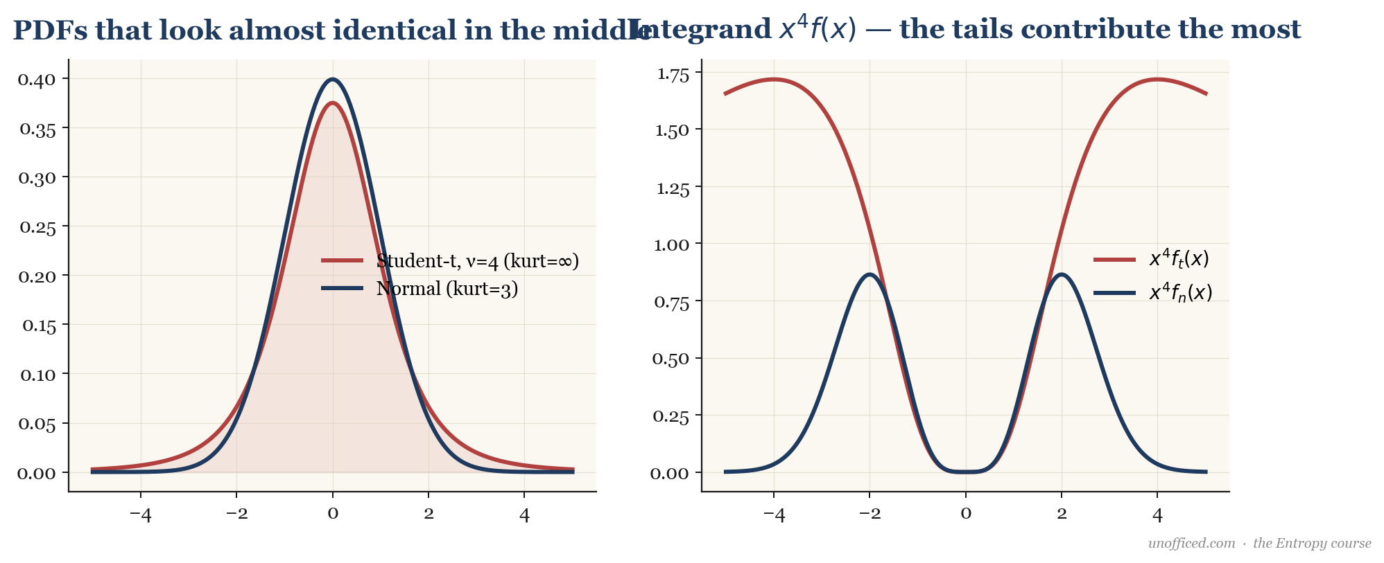
Where is the fourth central moment. The power of 4 is what gives kurtosis its sensitivity to outliers. A small number of large deviations from the mean, when raised to the fourth power, can dominate the numerator. This is why kurtosis specifically captures tail behaviour.
A standard normal distribution has a kurtosis of exactly 3. Because much of financial theory uses the Gaussian distribution as a benchmark, it is conventional to report excess kurtosis, which is simply kurtosis minus 3:
Under this convention:
- Mesokurtic: Excess kurtosis near 0 (e.g., the normal distribution). The tails are neither fat nor thin.
- Leptokurtic: Excess kurtosis > 0. The distribution is “fat-tailed” and typically more peaked around the mean than a normal distribution. Financial returns are almost universally leptokurtic.
- Platykurtic: Excess kurtosis < 0. The distribution is "thin-tailed," meaning outliers are very rare. This is uncommon in financial markets but can be seen in distributions like the uniform distribution.
Derivation for the Normal Distribution
The fact that a normal distribution has a kurtosis of 3 can be proven using its Moment Generating Function (MGF). For a standard normal variable , the MGF is . The k-th moment is the k-th derivative of the MGF evaluated at t=0.
The fourth moment is:
Since for a standard normal distribution , the kurtosis is .
The Student’s t-Distribution: A Better Model
The Student’s t-distribution is a leptokurtic distribution often used to model financial returns precisely because it has fatter tails. Its kurtosis depends on its degrees of freedom, :
For . In reality, the empirical data for NIFTY daily returns fits a t-distribution with somewhere between 5 and 8. Using the formula, this implies a theoretical excess kurtosis of to , which aligns well with observed data and confirms that “tail events” are far more likely than a Gaussian model admits.
Calculating Sample Kurtosis
In practice, we calculate kurtosis from a sample of N historical returns, . The formula for sample excess kurtosis is:
- Calculate Mean (): (-0.2%) or -0.002.
- Calculate Standard Deviation (): 1.76% or 0.0176.
- Calculate Fourth Central Moment (): Sum of divided by N.
The average is . - Calculate Kurtosis: .
- Calculate Excess Kurtosis: 2.57 – 3 = -0.43. This small, noisy sample happens to be platykurtic, driven by the single large outlier.
Empirical Kurtosis in Indian Markets
When we calculate excess kurtosis for Indian equity returns over long periods, it is consistently and significantly positive, confirming a leptokurtic world.
| Instrument | Typical Daily Excess Kurtosis | Notes |
|---|---|---|
| NIFTY 50 | 5 – 8 | Highly persistent fat tails. |
| BANKNIFTY | 6 – 12 | More volatile, higher kurtosis due to banking sector event risk. |
| Large-Cap Stocks (e.g., RELIANCE) | 4 – 15 | Varies by stock and sector. |
| Mid/Small-Cap Stocks | 15 – 40+ | Illiquidity and higher specific risk lead to extreme kurtosis. |
The effect is even more pronounced on shorter timeframes. For 15-minute returns, it is not uncommon to see excess kurtosis in the range of 20 to 50 for BANKNIFTY during volatile periods.
What Causes Fat Tails? Jump-Diffusion
The standard model of stock returns (Geometric Brownian Motion) assumes continuous price movement and produces normal returns. The observed kurtosis tells us this model is wrong. A better model, proposed by Robert Merton in 1976, is a jump-diffusion process. This model combines the standard continuous random walk with a Poisson process that generates sudden, large “jumps” in price. These jumps correspond to major news events: earnings surprises, RBI policy changes, geopolitical shocks, etc. It is these infrequent but large jumps that generate the fat tails we observe.
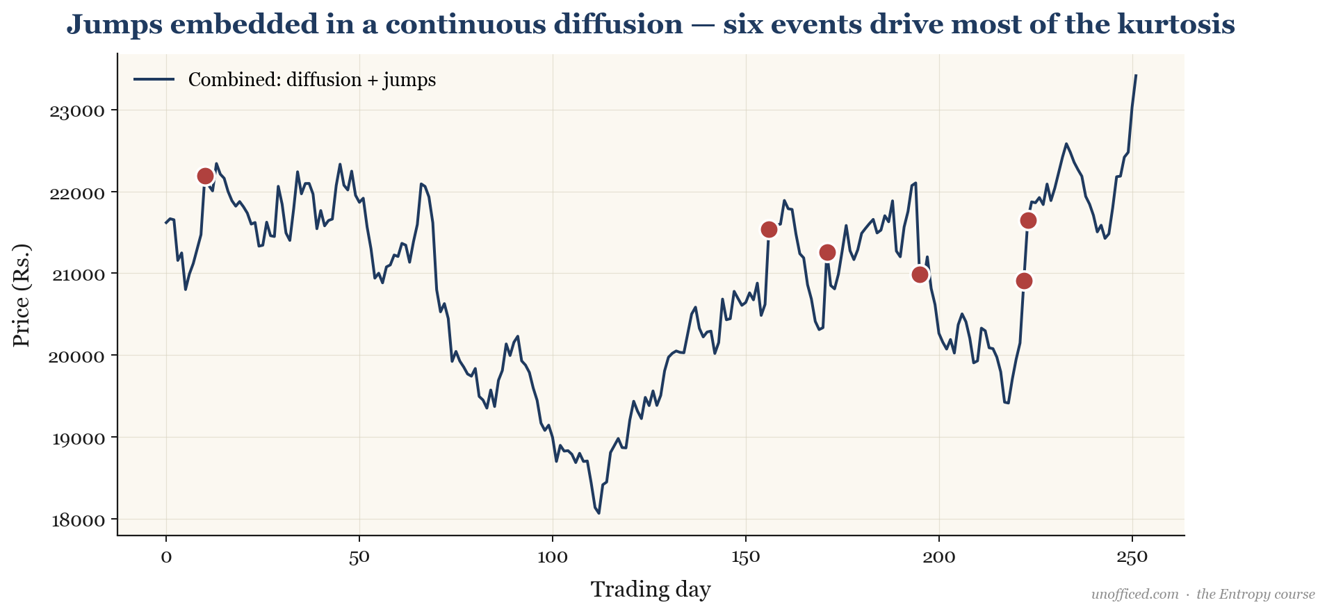
What this means for a trader: Your risk is not a smooth, continuous process. A significant portion of your long-term P&L will be determined by a handful of extreme days. Your risk management must account for the possibility of a sudden, discontinuous 10% gap down overnight, because the data shows it can and does happen.
Testing for Normality
The Jarque-Bera (JB) test is a formal statistical test that checks whether sample data has skewness and kurtosis matching a normal distribution. The test statistic is defined as:
Where N is the number of observations, S is the sample skewness, and K is the sample kurtosis. Under the null hypothesis of normality, the JB statistic has a chi-squared distribution with 2 degrees of freedom. For virtually any financial return series of sufficient length, the JB test statistic will be enormous, leading to a p-value of essentially zero and an unequivocal rejection of the normality assumption.
Implications for Trading and Risk Management
High kurtosis is not an academic curiosity; it has profound practical implications for risk management, strategy design, and option pricing.
Kurtosis Risk: The Illusion of Safety
Many strategies, particularly in the options selling space (like writing far out-of-the-money strangles), appear safe because they have low volatility and a high win rate. They generate small, steady profits for long periods, giving a false sense of security. However, these strategies often have extremely high negative skewness and high kurtosis. They are picking up pennies in front of a steamroller. The risk is not in the day-to-day fluctuations, but in the single catastrophic loss that wipes out years of gains. This is “kurtosis risk.”
Impact on Options Pricing: The Volatility Smile
The existence of the “volatility smile” in options markets is direct proof that market participants are aware of and price in kurtosis. The Black-Scholes-Merton model assumes returns are log-normally distributed (i.e., zero excess kurtosis). If this were true, the implied volatility for all options on the same underlying, with the same expiry, should be identical regardless of strike price. In reality, deep out-of-the-money and in-the-money options have a higher implied volatility than at-the-money options, creating a “smile” shape. This smile is the market’s way of charging a higher premium for puts and calls that would pay off during an extreme tail event. The smile is, in effect, the market price of kurtosis.
Sigma Events are Not Rare
High kurtosis means “sigma events” are much more common than a normal distribution suggests.
- A 3-sigma event is expected once every 370 occurrences in a normal world. For daily data, that’s about 1.5 years. In reality, NIFTY sees several such moves almost every year.
- A 6-sigma event is expected once in two million years in a normal world. Yet, we have seen multiple moves of this magnitude or greater on NIFTY in the last two decades alone (e.g., during the 2008 GFC, May 2009 election results, and the 2020 COVID crash).
Ignoring kurtosis leads to underestimating risk, using excessive leverage, and setting stop-losses that are systematically too tight for the instrument’s actual behaviour.
Summary
Kurtosis is a critical concept for any serious trader or quantitative analyst. It is the market’s way of reminding us that it is a wilder place than textbook models suggest.
- Kurtosis () is the fourth standardized moment, measuring the “tailedness” of a distribution and the frequency of extreme outliers.
- Financial returns are leptokurtic (“fat-tailed”), exhibiting positive excess kurtosis ().
- This is likely caused by discontinuous “jumps” in price, as described by jump-diffusion models.
- High kurtosis causes standard statistical tools to underestimate the frequency and magnitude of large price moves. Events that are “6-sigma” in a normal world happen with unsettling regularity in real markets.
- It has direct, practical consequences, creating “kurtosis risk” in seemingly low-volatility strategies and giving rise to the volatility smile in option prices.
Understanding kurtosis is the first step toward appreciating tail risk. The next is to build systems and risk management frameworks that are robust to this feature of financial markets, particularly when it comes to position sizing and avoiding strategies that have a high probability of ruin.
Further Reading
- Taleb, Nassim Nicholas. The Black Swan: The Impact of the Highly Improbable. A foundational, non-technical exploration of fat tails and their consequences.
- Wilmott, Paul. Paul Wilmott on Quantitative Finance. Provides a rigorous but practical overview of the mathematical models used in finance, including critiques of their limitations.
- Merton, Robert C. (1976). “Option pricing when underlying stock returns are discontinuous.” Journal of Financial Economics. The original academic paper proposing the jump-diffusion model.
- Ross, Sheldon M. A First Course in Probability. An excellent textbook for understanding the mathematical foundations of probability theory that underpin all quantitative finance.