Random Variable

In financial markets, a **random variable** is a quantity whose value is a numerical outcome of a random process. The price of NIFTY at tomorrow’s close, the number of trades stopped out in a week, or the maximum drawdown a strategy will suffer next month are all random variables. Understanding their nature is critical for modelling.
Formal Definition of a Random Variable
More formally, a random variable is a function that maps outcomes from a sample space, , to the set of real numbers, . If is our random variable, then . For an outcome (e.g., a specific sequence of future price movements), is the corresponding numerical value (e.g., the final return).
This framework is governed by three fundamental axioms of probability, first laid down by Andrey Kolmogorov:
- Non-negativity: The probability of any event is non-negative: .
- Normalisation: The probability of the entire sample space is 1: . Some outcome must occur.
- Sigma-additivity: For any countable collection of mutually exclusive events (i.e., for ), the probability of their union is the sum of their individual probabilities: .
The most fundamental distinction in characterising a random variable is whether it is discrete or continuous.
Discrete vs. Continuous Random Variables
A discrete random variable can only take a countable number of distinct values. For each possible value , we can assign a probability using a Probability Mass Function (PMF), such that . The sum of all probabilities must be exactly 1: . Think of counts: the number of winning trades out of 10, the number of times a stock breaches its upper Bollinger Band in a month, or the number of ticks a price moves in an hour. These are all discrete outcomes.
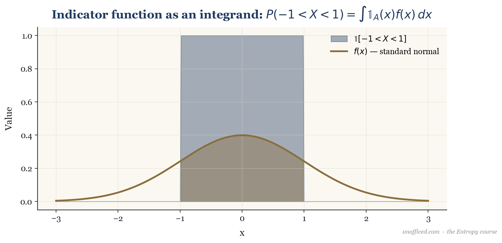
A continuous random variable, in contrast, can take any value within a given range. We cannot assign a non-zero probability to a single point. Instead, we define a Probability Density Function (PDF), , which describes the relative likelihood of a variable taking on a given value. The probability of the variable falling within an interval is the area under the curve, found by integration:
, which is 1 if is in the interval and 0 otherwise. The probability is the expected value of this indicator function.
Stock Prices are Discrete; Returns are Continuous
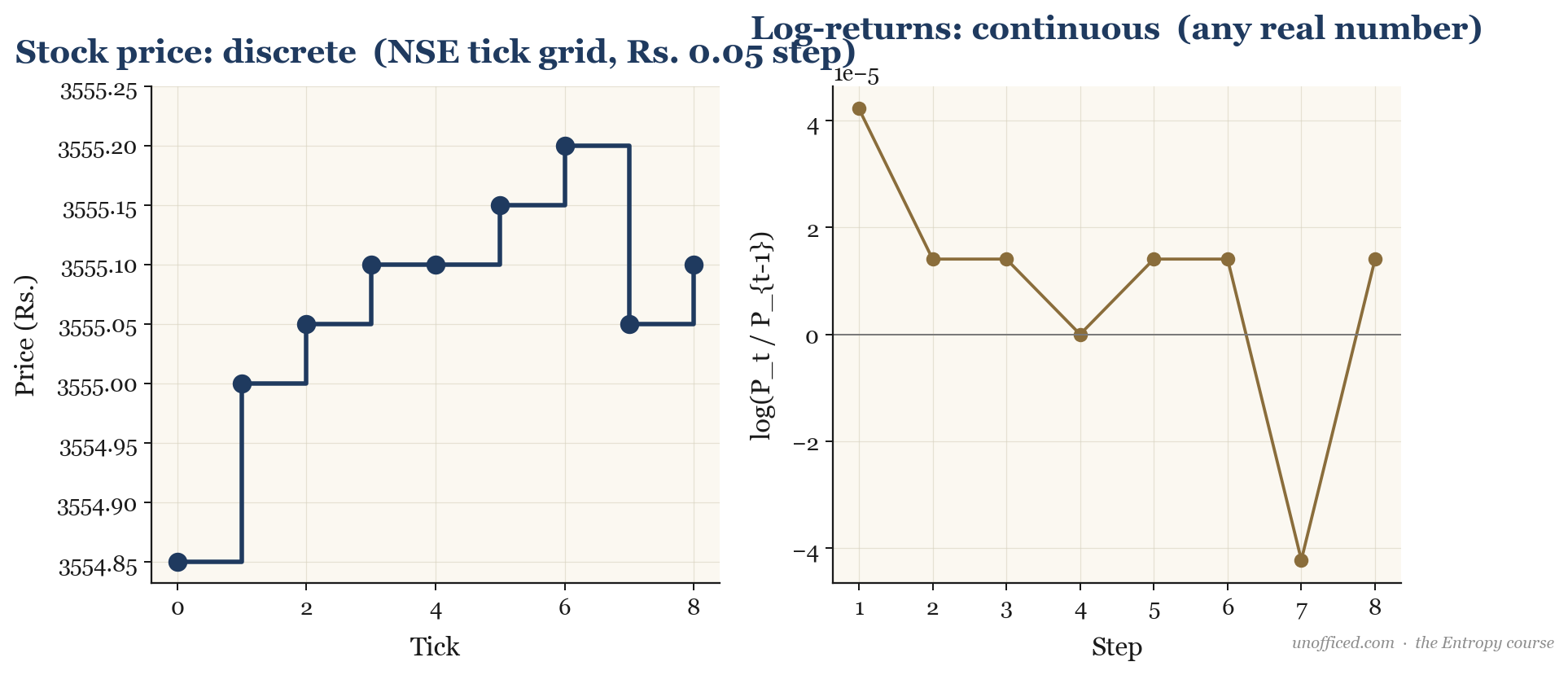
This distinction is not merely academic; it has practical consequences in financial data analysis. Stock prices on the National Stock Exchange (NSE) are discrete. For stocks priced at or above Rs. 250, the minimum price movement, or “tick size,” is Rs. 0.05. A stock can be priced at Rs. 1,000.05 or Rs. 1,000.10, but never Rs. 1,000.073. The set of possible prices is a grid, not a continuum. This has implications for high-frequency strategies but is less critical for daily or weekly analysis.
However, the returns calculated from these prices are treated as continuous for modelling purposes. Whether you calculate a simple return or a log-return , the result is a real number that can, in theory, take any value in a range. The move from a discrete price grid to a continuous world of returns is a foundational concept for quantitative analysis.
What this means for a trader: The discreteness of prices means your limit orders can only be placed on specific price levels. However, your risk and performance models will almost always be based on continuous returns, which is a valid and powerful abstraction.
Why Use Log-Returns?
While simple returns are intuitive, log-returns () are overwhelmingly preferred in quantitative finance for three key reasons:
- Additivity: The log-return over multiple periods is simply the sum of the individual log-returns for each period. The log-return from day 1 to day 3 is . Simple returns do not have this convenient property; they must be geometrically compounded.
- Symmetry: Log-returns treat gains and losses symmetrically. A simple return of +10% (price goes from 100 to 110) requires a -9.09% return to get back to 100. In log-space, these are symmetric: and . This avoids analytical bias.
- Distributional Assumptions: Many financial models, including the Black-Scholes model for options pricing, assume that log-returns of the underlying asset are normally distributed. This makes them mathematically tractable, forming the bedrock of quantitative finance.
Moments of a Distribution: Expectation and Variance
To describe a random variable, we use its “moments.” The first moment is its Expected Value (or mean), which is the long-run average value of its realisations.
Expectation
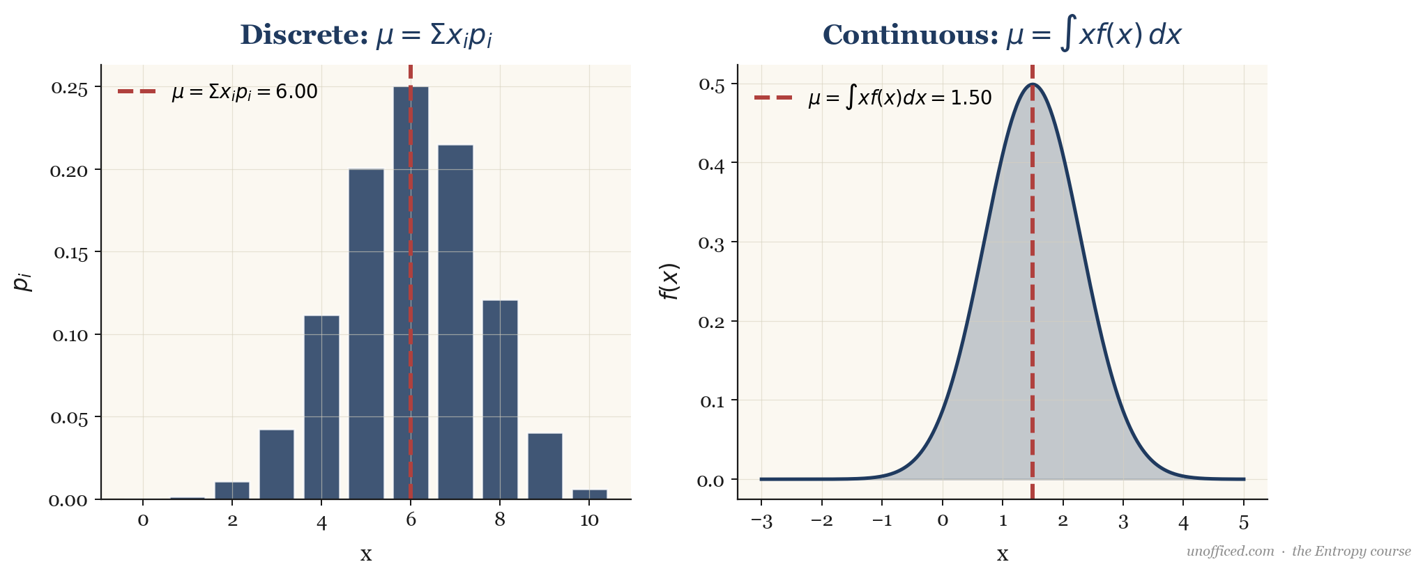
For a discrete variable with PMF , the expectation is the probability-weighted sum of all possible values:
For a continuous variable with PDF , the expectation is the integral of weighted by its probability density:
Expectation is a linear operator. For random variables and constants , we have Linearity of Expectation:
This property is incredibly powerful and holds regardless of whether X and Y are independent.
Variance
The second central moment is the Variance, which measures the dispersion or “spread” of the distribution around its mean. It is defined as the expected value of the squared deviation from the mean, .
A more computationally convenient formula for variance can be derived from the definition:
The square root of the variance, , is the standard deviation, which is expressed in the same units as the random variable itself and is the most common measure of financial risk.
What this means for a trader: The expected return () tells you what you can expect to make on average per trade, while the standard deviation () tells you how volatile or risky that return stream is. The ratio of these two, , is the foundation of the Sharpe Ratio, a key performance metric.
Joint Distributions, Covariance, and Correlation
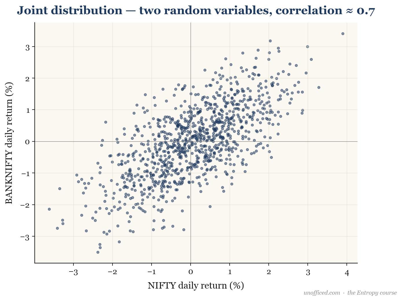
Often, we need to model the relationship between two or more random variables. For two variables and , we use a joint probability distribution. The Covariance measures how they move together.
A positive covariance means the variables tend to move in the same direction, while a negative covariance means they move in opposite directions. However, the magnitude of covariance is hard to interpret. We normalise it to get the Correlation Coefficient, (rho).
The Cauchy-Schwarz inequality guarantees that . A correlation of +1 implies perfect linear co-movement, -1 implies perfect inverse linear co-movement, and 0 implies no linear relationship.
For example, NIFTY 50 and BANKNIFTY are highly correlated because banking stocks constitute a large portion of the NIFTY 50 index. Their daily returns often show a correlation coefficient around +0.8 to +0.9.
| Day | Return R (%) | Return I (%) |
|---|---|---|
| 1 | +0.5 | +1.0 |
| 2 | -0.2 | -0.4 |
| 3 | +1.1 | +0.8 |
| 4 | -0.8 | -1.2 |
| 5 | +0.4 | +0.6 |
First, calculate the mean returns: and .
The sample covariance is .
.
Since the covariance is positive, it indicates they tend to move together over this period.
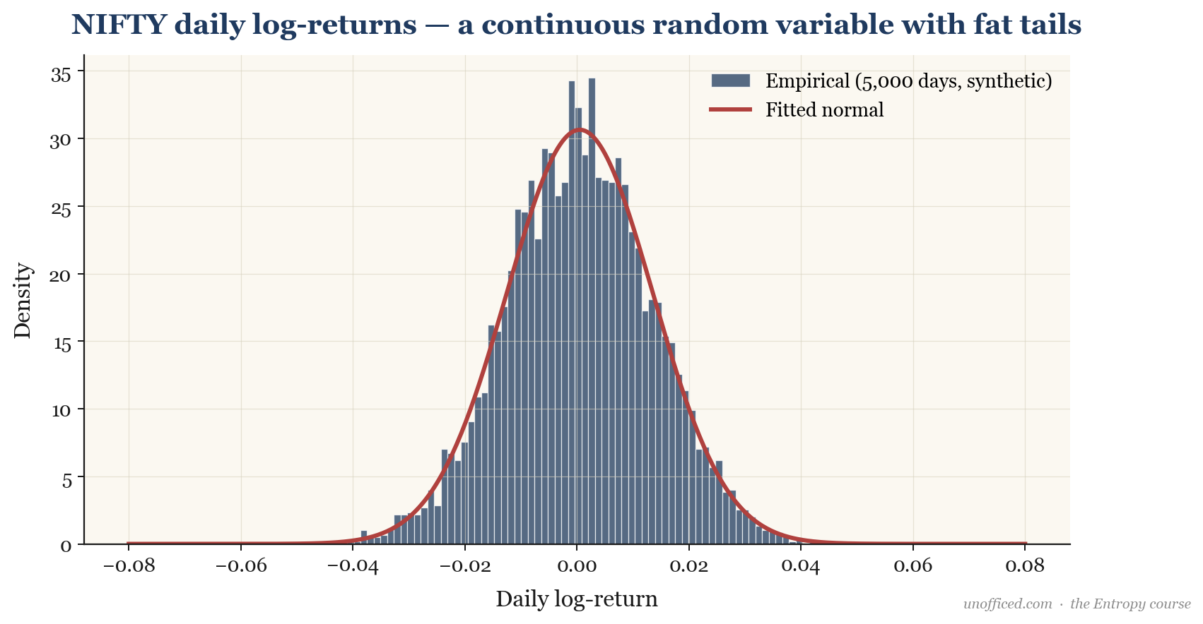
The Empirical Distribution of NIFTY Log-Returns
If we take historical data and plot a histogram of daily log-returns, we get what is called an “empirical distribution.” This shows us what the random variable has actually looked like in the past. Below is a histogram of 5,000 simulated daily log-returns for NIFTY, with a fitted Normal (Gaussian) distribution overlaid.
Key Theorems: LLN, CLT, and Ergodicity
Two major theorems form the foundation of statistical inference:
- The Law of Large Numbers (LLN): States that the average of the results obtained from a large number of independent and identically distributed (i.i.d.) random variables will be close to the true expected value. Your backtest’s average P&L per trade approaches the true expectancy of your strategy as the number of trades grows.
- The Central Limit Theorem (CLT): States that the sum (or average) of a large number of i.i.d. random variables, each with a finite mean and variance, will be approximately normally distributed, *regardless of the underlying distribution*. This is why the normal distribution is so ubiquitous.
Finally, a crucial concept for backtesting is ergodicity. A process is ergodic if its time-average is the same as its ensemble average. In trading, this means assuming that the statistical properties of the market (like mean return and volatility) observed over a long period in the past (your backtest) are the same as the properties one would find by looking at many different parallel universes of market evolution at a single point in time. If the market regime changes drastically, this assumption can fail, and past performance becomes no guarantee of future results.
Summary
- A random variable is a function mapping random outcomes to numerical values, governed by the axioms of probability.
- Discrete random variables are counted (e.g., number of trades), while continuous random variables are measured (e.g., log-returns).
- Stock prices are discrete, moving in fixed tick sizes, but the returns calculated from them are modelled as continuous.
- Log-returns are preferred over simple returns for their properties of additivity, symmetry, and convenient distributional assumptions.
- A distribution’s properties are described by its moments, like the mean (Expectation) and the Variance.
- Covariance and Correlation measure how two random variables move in relation to each other.
- The actual (empirical) distribution of NIFTY log-returns is approximately normal but exhibits “fat tails,” meaning extreme outcomes are more common than a pure normal distribution would suggest.
- The Law of Large Numbers and Central Limit Theorem are pillars of statistical inference, but their application requires careful consideration of assumptions like ergodicity.
Understanding returns as a continuous random variable is the first step. The next lesson builds on this by formalizing the concept of continuous compounding and showing why log-returns are its natural language.
Further Reading
- Ross, Sheldon. A First Course in Probability. A classic and accessible introduction to probability theory.
- Taleb, Nassim Nicholas. The Black Swan: The Impact of the Highly Improbable. A seminal work on the importance of fat tails and extreme events in finance and beyond.
- Wilmott, Paul. Paul Wilmott on Quantitative Finance. A comprehensive practitioner’s guide to the mathematics of financial markets.