Probability Distribution

A probability distribution describes the likelihood of each possible outcome for a random variable. It is a fundamental concept in statistics that tells us how probabilities are distributed over the possible values the variable can take. Understanding distributions allows us to move from simply describing data to quantifying uncertainty and making probabilistic forecasts, the very core of a quantitative trading endeavour.
The Language of Uncertainty: PMF, PDF, and CDF
In our previous lesson on random variables, we distinguished between discrete and continuous variables. This distinction gives rise to two families of probability distributions, each with its own mathematical language.
Discrete Distributions: The Probability Mass Function (PMF)
A discrete random variable has a finite or countably infinite number of possible values, like the number of ticks a stock moves in a minute. Its distribution is described by a Probability Mass Function (PMF), which assigns a specific probability to each exact outcome.
For a valid PMF, two conditions must hold:
- for all possible outcomes .
- The sum of all probabilities must equal 1: .
- P(X = +5) = 0.30
- P(X = 0) = 0.50
- P(X = -5) = 0.20
This is a valid PMF as the probabilities are non-negative and sum to 1. The expected outcome (mean) is . Our expectation is a slight positive drift post-announcement.
Continuous Distributions: The Probability Density Function (PDF)
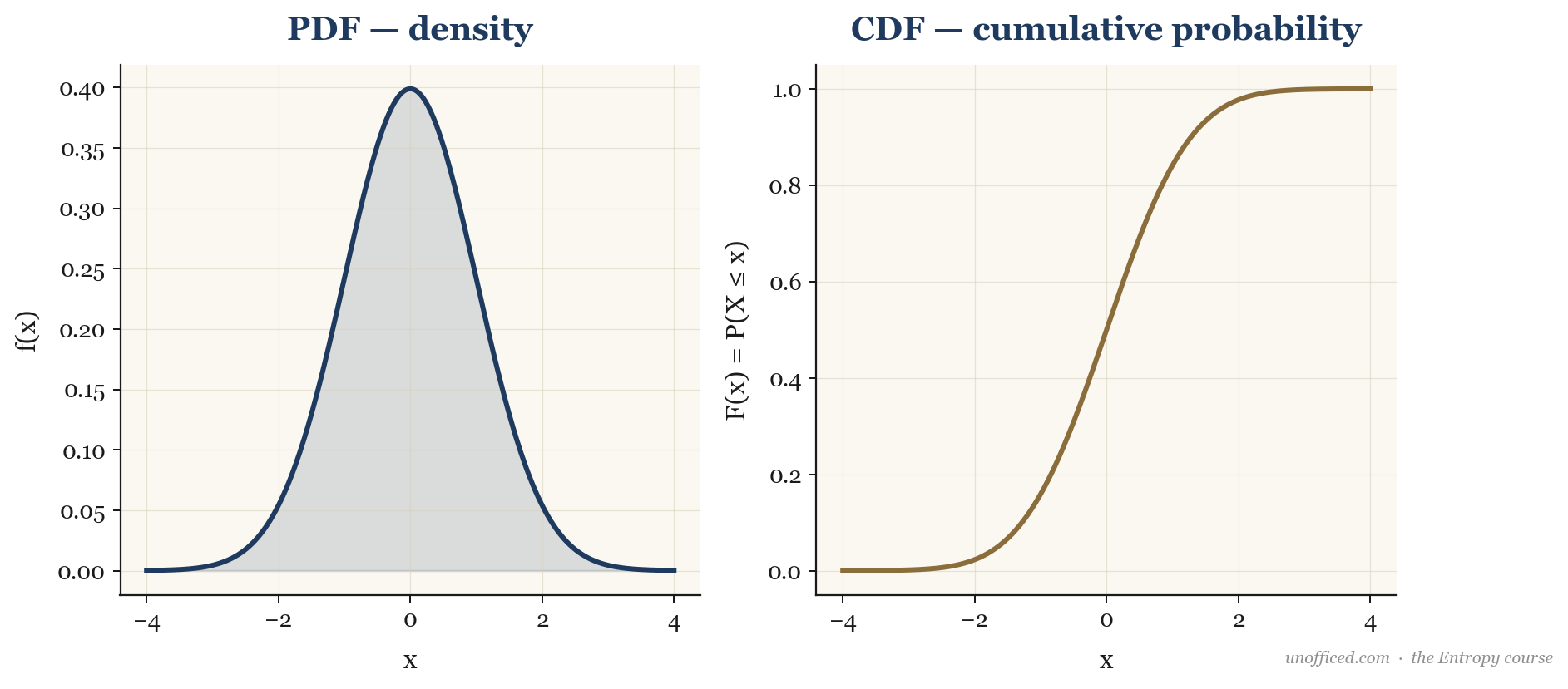
A continuous random variable can take any value within a given range, such as the daily percentage return of NIFTY. We cannot assign a non-zero probability to a single point, as there are infinitely many points. Instead, we describe its distribution using a Probability Density Function (PDF), denoted . The PDF’s value is not a probability; it represents probability *density*. To get a probability, we must integrate the PDF over an interval.
.
The Universal Descriptor: The Cumulative Distribution Function (CDF)
For both discrete and continuous variables, the Cumulative Distribution Function (CDF), denoted , provides a unified way to describe the distribution. It gives the total probability that the variable takes on a value less than or equal to .
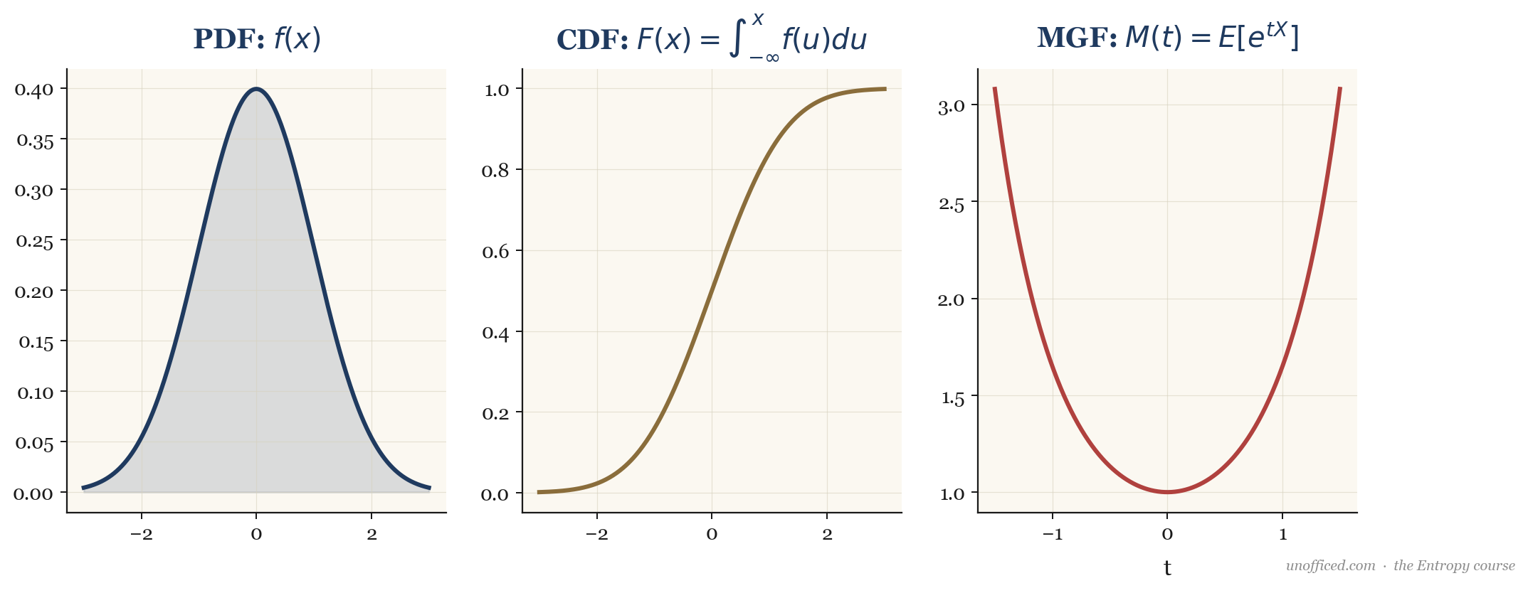
For a continuous variable, , and consequently, the PDF is the derivative of the CDF: . The CDF is non-decreasing and always ranges from 0 to 1, making it one of the most fundamental objects in probability theory.
What this means for a trader: The CDF is directly applicable to risk management. The probability of a loss exceeding some value is , is defined as the expected value of :
The magic of the MGF lies in its Taylor series expansion:
By differentiating the MGF with respect to and evaluating at , we can extract the raw moments ().
For example, the first moment (mean) is , and the second raw moment is , from which we get the variance: .
The Characteristic Function
Not all distributions have a well-defined MGF (it might not converge). A more universally applicable tool is the Characteristic Function (CF), , which always exists. It’s defined using a complex exponential:
The CF has similar properties to the MGF and is central to advanced probability theory, particularly for working with sums of random variables and distributions like the Cauchy that lack finite moments.
Moments: The Four Key Descriptors
Distributions are often summarised by a set of parameters known as moments. These describe the shape and location of the distribution. For traders, the first four are the most critical for understanding risk and return.
- Mean (): The first moment about the origin. It represents the expected value or the “center of mass” of the distribution. .
- Variance (): The second central moment (i.e., moment about the mean). It measures the dispersion or spread of the data around the mean. . Its square root, , is the standard deviation.
- Skewness (): The third standardized moment, measuring the asymmetry of the distribution. A negative skew indicates a longer or fatter tail on the left side. We discuss this in detail in the lesson on Skewness.
- Kurtosis (): The fourth standardized moment, measuring the “tailedness” or propensity for extreme outliers compared to a normal distribution. This is covered in the lesson on Kurtosis.
The Empirical Distribution
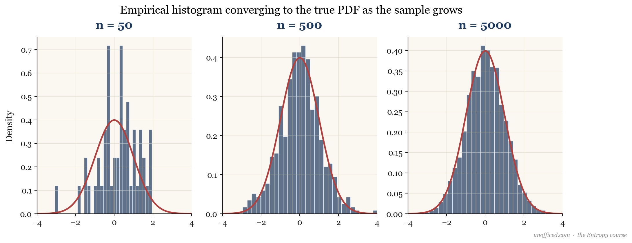
In practice, we never know the true underlying probability distribution of a financial random variable like the daily returns of ICICI Bank. All we have is a finite sample of historical data. From this sample, we can construct an empirical distribution. A histogram is the most common way to visualise the empirical PDF.
The Law of Large Numbers gives us theoretical comfort: as we collect more data (i.e., as the sample size ), the empirical distribution will converge to the true, unknown underlying distribution.
What this means for a trader: All our backtesting and risk modelling is done on the empirical distribution. The core assumption is that this historical distribution is a good proxy for the future distribution. This assumption (stationarity) often breaks down, especially during market regime changes, which is a primary source of model failure.
The Myth of Normality in Markets
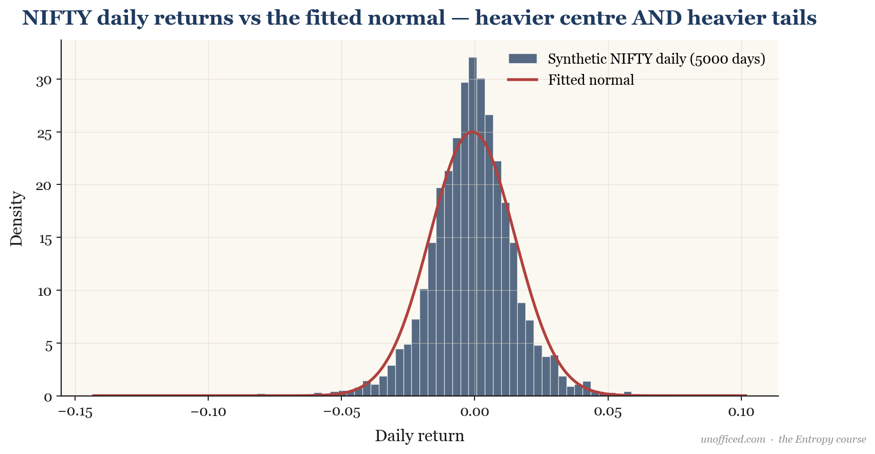
The normal (or Gaussian) distribution is the cornerstone of modern finance, underpinning models like Black-Scholes. It is mathematically elegant and provides a decent first approximation for financial returns. However, the strict assumption of normality is demonstrably false and dangerously misleading.
When we plot a histogram of NIFTY daily returns against a fitted normal distribution, we see a close match near the center. But the empirical distribution shows two critical deviations:
- Fat Tails (Leptokurtosis): The real-world distribution produces far more extreme positive and negative returns than a normal distribution would predict. The tails of the distribution are “fatter,” meaning -5% or +5% days happen more often than the Gaussian model allows.
- Negative Skew: Large negative returns (crashes) are slightly more frequent and severe than large positive returns (rallies), creating a slight leftward lean in the distribution.
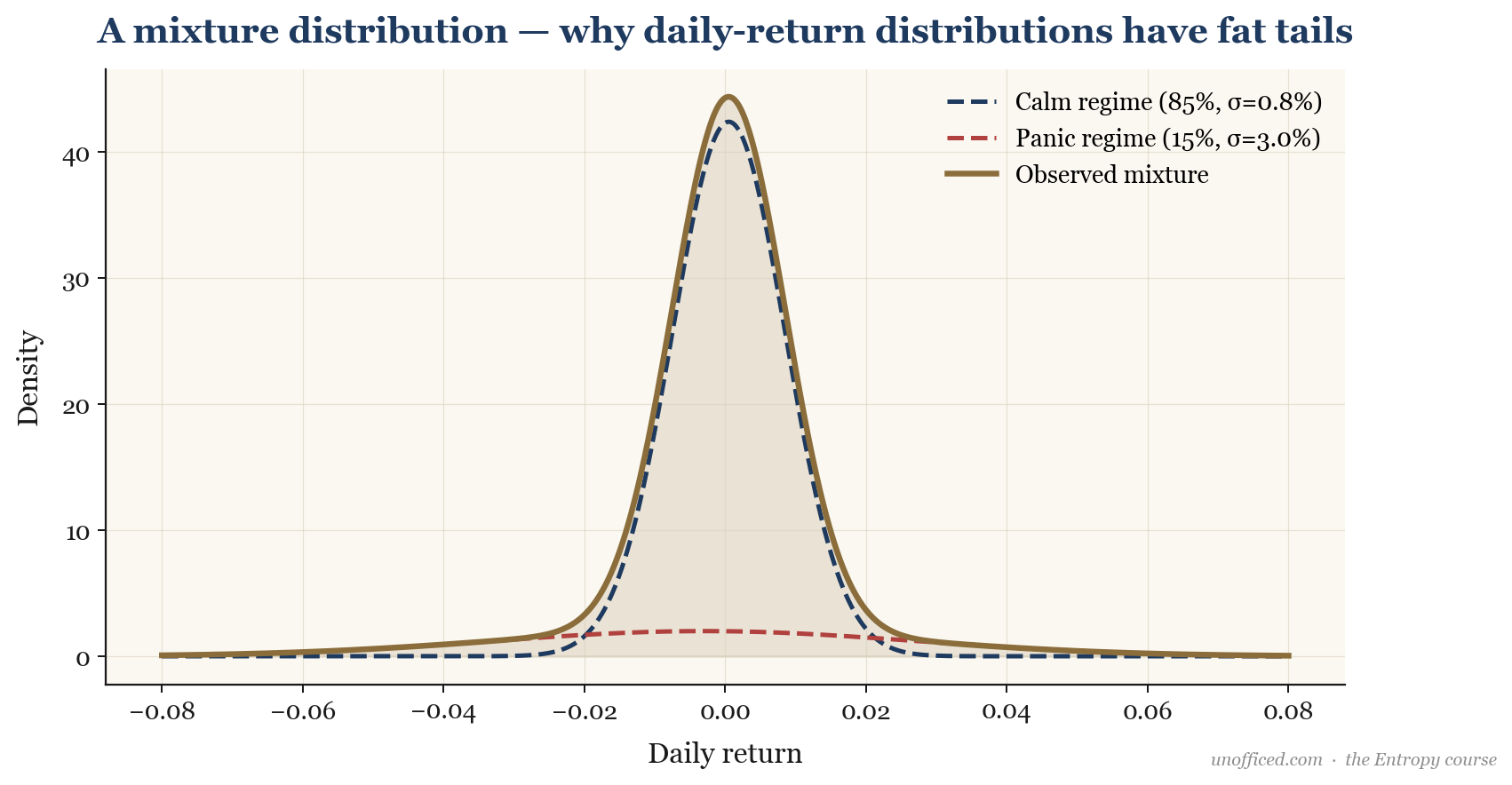
Explaining Fat Tails: Mixture Distributions
Why do returns have fat tails? One powerful explanation is the concept of a mixture distribution. The market doesn’t operate in a single, static mode. Instead, it switches between different “regimes”—typically a low-volatility “calm” regime and a high-volatility “panic” regime.
The overall distribution of returns is a probability-weighted average (a mixture) of the distributions from these two regimes. The panic regime, even if it occurs only 5-10% of the time, contributes its high variance to the mixture, fattening the tails of the combined distribution.
This model intuitively captures market reality: long periods of quiet punctuated by short, violent bursts of activity. This is the mathematical source of fat tails.
Diagnosing Distributions: The Q-Q Plot
How can we visually check if our data fits a certain theoretical distribution (e.g., normal)? The histogram is a start, but a more rigorous tool is the Quantile-Quantile (Q-Q) plot.
This plot compares the quantiles of our empirical data against the theoretical quantiles of the distribution we are testing.
- If the data is a perfect match for the theoretical distribution, the points on the Q-Q plot will lie perfectly on a 45-degree line.
- Deviations from the line indicate a mismatch. For financial returns plotted against a normal distribution, the classic pattern is an “S” shape. The tails of the data (both left and right) are more extreme than the normal quantiles, causing the points to curve away from the straight line at both ends. This is the visual signature of fat tails.
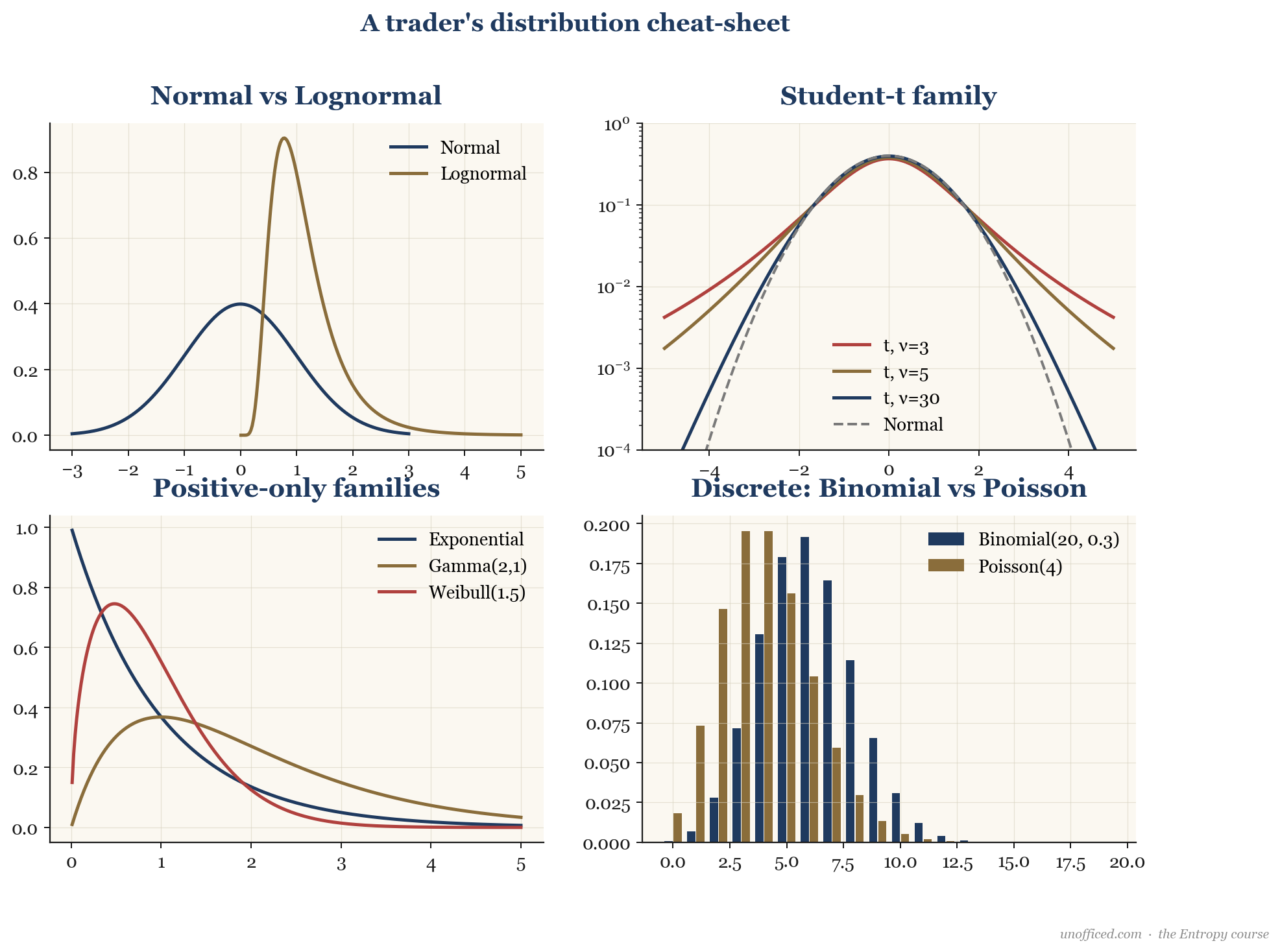
The Quant Trader’s Distribution Cheat-Sheet
Traders and quants use a menagerie of distributions to model different market phenomena. Choosing the right one is key to building robust models.
| Distribution | Use Case in Trading | Key Parameters |
|---|---|---|
| Normal | A flawed but foundational model for daily/weekly returns. Central to Black-Scholes. | Mean (), Std. Dev. () |
| Log-normal | Modelling asset prices (), which cannot be negative. If log-returns are normal, prices are log-normal. | of the log-returns. |
| Student’s t | A superior model for returns that explicitly incorporates fat tails. A common replacement for the normal. | Degrees of Freedom (). As , it becomes normal. between 3 and 5 is common for returns. |
| Binomial | Modelling a number of “successes” in a fixed number of independent trials (e.g., number of up-days in a week). | Number of trials (), success probability (). |
| Poisson | Modelling the number of events occurring in a fixed interval of time/space (e.g., number of trades in a 1-minute bar). | Rate parameter (). |
| Exponential | Modelling the time *between* events in a Poisson process (e.g., time between two consecutive large trades). | Rate parameter (). |
| Pareto / Power-law | Modelling “black swan” events, the size of market crashes, wealth distribution. Describes “80/20” phenomena. | Shape parameter / exponent (). |
| Weibull / Gamma | Flexible distributions for modelling durations, such as the time until a stop-loss is hit or a trade is closed. | Shape (), Scale (). |
Advanced Concepts
Entropy: Measuring “Surprise”
In information theory, the entropy of a distribution measures its “surprise” or uncertainty. A uniform distribution, where all outcomes are equally likely, has maximum entropy. A distribution concentrated on a single value has zero entropy. For a trader, high entropy implies low predictability.
Copulas: Modelling Dependence Beyond Correlation
Correlation only measures linear relationships. Markets, however, exhibit complex, non-linear dependencies, especially during crises (e.g., all asset classes fall together). Copulas are functions that separate a multivariate distribution into its marginal distributions (for each variable) and a structure that describes their dependence. This allows for far more sophisticated modelling of portfolio risk than simple correlation matrices.
Further Reading
- A First Course in Probability by Sheldon Ross. The canonical undergraduate text for a rigorous introduction.
- The Black Swan: The Impact of the Highly Improbable by Nassim Nicholas Taleb. A crucial non-technical book on the importance of fat tails and the failure of Gaussian models in the real world.
- Analysis of Financial Time Series by Ruey S. Tsay. An advanced, comprehensive guide to the statistical properties of market data.
Summary
- A probability distribution quantifies the likelihood of all outcomes for a random variable, using a PMF for discrete variables and a PDF for continuous ones. The CDF, , is a universal descriptor.
- Moments like mean, variance, skewness, and kurtosis summarise a distribution’s shape. Generating functions (MGF, CF) provide a powerful way to derive these moments.
- Stock returns are not normally distributed. They empirically exhibit “fat tails” (leptokurtosis) and negative skew, often explained by mixture distributions representing different market regimes.
- Relying on the normal distribution for risk management is perilous. Alternatives like the Student’s t-distribution and diagnostic tools like the Q-Q plot are essential for realistic modelling.
- A professional quant uses a wide range of distributions to model specific market phenomena, from Poisson for event counts to Pareto for extreme tail events.