Find the Equilibrium Matrix in Markov Chain using Python in Indian Stock Market

Find the Equilibrium Matrix in Markov Chain using Python in Stock Market
Before We discuss further, Please read make sure You have read the previous articles in this following order –
- Part I – Stochastic Modeling
- Part II – Application of Markov Chains in Stock Market
- Part III – Markov Chains in Stock Market Using Python – Getting Transition Matrix
- Part IV – How to do Random Walk using NSEPython in Indian Stock Market
- Part V – Markov Chain and Linear Algebra – Calculation of Stationary Distribution using Python
Recap on Getting Transition Matrix in Markov Chain Using Python
Let’s follow the path shown in Markov Chains in Stock Market Using Python – Getting Transition Matrix, Here is the sum of the whole python code so far to get Transition Matrix –
					symbol = "NIFTY 50"
days = 1000
end_date = datetime.datetime.now().strftime("%d-%b-%Y")
end_date = str(end_date)

start_date = (datetime.datetime.now()- datetime.timedelta(days=days)).strftime("%d-%b-%Y")
start_date = str(start_date)

df=index_history("NIFTY 50",start_date,end_date)

df["state"]=df["CLOSE"].astype(float).pct_change()
df['state']=df['state'].apply(lambda x: 'Upside' if (x > 0.001) else ('Downside' if (x<=0.001) else 'Consolidation'))

df['priorstate']=df['state'].shift(1)

states = df [['priorstate','state']].dropna()
states_matrix = states.groupby(['priorstate','state']).size().unstack().fillna(0)

transition_matrix= states_matrix.apply(lambda x: x/float(x.sum()),axis=1)
print(transition_matrix)
Output –
					state          Downside    Upside
priorstate
Consolidation  0.000000  1.000000
Downside       0.638821  0.361179
Upside         0.554307  0.445693
Forecasting Futures Probabilities of States using Python
Now, We will walk the sections discussed in Markov Chain and Linear Algebra – Calculation of Stationary Distribution using Python again but this time using Python. Remember this diagram?
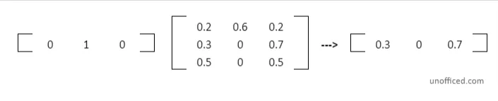
Let’s consider time as t. Now, We will see observe other probability matrices.
In case You are confused with the terms of “Transition Matrix” and “Probability Matrix” again. “Transition Matrix” is the probability matrix at t=0. It shows the probability at t=0, right?
So, Let’s build the Markov Chain by multiplying this transition matrix by itself to obtain the probability matrix in t=1 which would allow us to make one-day forecasts.
					t_0 = transition_matrix.copy()
t_1 = round(t_0.dot(t_0),4)
t_1
Output –
					---------------------------------------------------------------------------
ValueError                                Traceback (most recent call last)
<ipython-input-11-4c583b2519ce> in <module>
      1 t_0 = transition_matrix.copy()
----> 2 t_1 = round(t_0.dot(t_0),4)
      3 t_1

\python39\lib\site-packages\pandas\core\frame.py in dot(self, other)
   1242             common = self.columns.union(other.index)
   1243             if len(common) > len(self.columns) or len(common) > len(other.index):
-> 1244                 raise ValueError("matrices are not aligned")
   1245
   1246             left = self.reindex(columns=common, copy=False)

ValueError: matrices are not aligned
The dot function only works if the Matrix is 2x2 or 3x3. As The “consolidation” state’s column in the last is filled with 0,0,0. Our 3x3 matrix becomes 3x2. So, Let’s just remove the consolidation state as it has so low outcome.
					symbol = "NIFTY 50"
days = 1000
end_date = datetime.datetime.now().strftime("%d-%b-%Y")
end_date = str(end_date)

start_date = (datetime.datetime.now()- datetime.timedelta(days=days)).strftime("%d-%b-%Y")
start_date = str(start_date)

df=index_history("NIFTY 50",start_date,end_date)

df["state"]=df["CLOSE"].astype(float).pct_change()
df['state']=df['state'].apply(lambda x: 'Upside' if (x > 0) else 'Downside' )

df['priorstate']=df['state'].shift(1)

states = df [['priorstate','state']].dropna()
states_matrix = states.groupby(['priorstate','state']).size().unstack().fillna(0)

transition_matrix= states_matrix.apply(lambda x: x/float(x.sum()),axis=1)
print(transition_matrix)
Output –
					state       Downside    Upside
priorstate
Downside    0.595238  0.404762
Upside      0.515152  0.484848
					t_0 = transition_matrix.copy()
t_1 =t_0.dot(t_0)
t_1
Output –
					state   	Downside	Upside
priorstate
Downside	0.562822	0.437178
Upside  	0.556408	0.443592
The Initial Transition Matrix
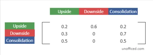
Just putting the image of Transition Matrix to help to visualize!
Construction of the Markov Chain Using Python
Just syncing with the last chapter where we discussed this in Linear Algebra section, Here the π_0 = t_0 = A.
Now, We need to extend the Markov Chain similarly. You can refer the below diagram if it helps to recall.
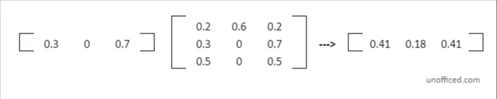
So, π_1.A =
Similarly, π_2.A =
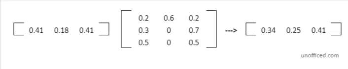
If we continue multiplying the transition matrix that we have obtained in t=1 by the original transition matrix in t0, we obtain the probabilities in time t=2. Let’s find the transition matrix at t=2 and t=3 and so on in a similar manner.
					t_2 = t_0.dot(t_1)
t_2
Output –
					state   	Downside	    Upside
priorstate
Downside	0.560226	0.439774
Upside  	0.559712    0.440288
					t_3 = t_0.dot(t_2)
t_3
Output –
					state	    Downside	Upside
priorstate
Downside	0.560018	0.439982
Upside	    0.559977	0.440023
Let’s Normalize –
					import numpy as np
pd.DataFrame(np.linalg.matrix_power(t_0,4))
Output –
					#
    0	        1
0	0.560018	0.439982
1	0.559977	0.440023
The result is a new transition matrix.
The values in this matrix represent the probabilities of transitioning from one state to another after four steps.
Matrix Exponentiation
In the Markov Chain theory, multiplying the transition matrix by itself (a process known as matrix exponentiation) corresponds to advancing the process forward in time. In this case, it’s being advanced four steps into the future.
This numpy technique provides us with matching outcomes. If you’re familiar with Linear Algebra principles, this will make sense since our π_0 = t_0 = A. Here, we are elevating the initial transition matrix to the power of n+1 days to achieve the desired result.
Hence, the expression becomes
t_n = pd.DataFrame(np.linalg.matrix_power(t_0,n+1))
The result t_n gives us a new transition matrix that represents the transition probabilities n steps into the future.
Finding Equilibrium Matrix using Python
To uncover the equilibrium matrix, we aim to find a state where the transition probabilities stabilize, showing no further change. This stable state is achieved when, upon further iterations, the transition matrix remains unchanged.
Input –
					t_0 = transition_matrix.copy()

t_m = t_0.copy()
t_n = t_0.dot(t_0)

i = 1
while(not(t_m.equals(t_n))):
    i += 1
    t_m = t_n.copy()
    t_n = t_n.dot(t_0)

print("Equilibrium Matrix Number: " + str(i))
print(t_n)
Output –
					Equilibrium Matrix Number: 16
state       Downside  Upside
priorstate
Downside        0.56    0.44
Upside          0.56    0.44
So, t = 16, We get our equilibrium matrix.
The code provided demonstrates an iterative process in Python, where we continually multiply the transition matrix by itself until we reach this stable state, which is the equilibrium matrix.
Here’s the breakdown of the code provided:
Initial Setup:
- t_0 is initialized as a copy of the transition matrix.
- t_m and t_n are both initialized as t_0 and the result of multiplying t_0 with itself (t_0.dot(t_0)), respectively.
- A counter i is set to 1 to keep track of the iterations.
					t_0 = transition_matrix.copy()
t_m = t_0.copy()
t_n = t_0.dot(t_0)
i = 1
Iterative Process:
- A while loop is initiated, which continues until the matrices t_m and t_n are equal.
- Within each iteration, t_m is updated to t_n, and t_n is updated to the result of multiplying t_n with t_0.
- The counter i is incremented by 1 with each iteration.
					while(not(t_m.equals(t_n))):
    i += 1
    t_m = t_n.copy()
    t_n = t_n.dot(t_0)
Output:
Once the loop exits, indicating that the equilibrium matrix is found, the number of iterations and the equilibrium matrix are printed out.
In this equilibrium matrix, regardless of the prior state (Upside or Downside), the probabilities for the next state being Downside or Upside are 0.56 and 0.44, respectively.
What is the meaning of Equilibrium Matrix?
The Equilibrium Matrix reflects a stable state in a Markov Chain where the probabilities of transitioning between states cease to change with further iterations. It represents a long-term view of how states interact within the system. According to Markov Chain theory, once reached, this equilibrium remains consistent across future data points.
To illustrate this, the provided code executes an analysis over an extended period, akin to our previous random walk analysis, but this time over 9209 days.
					symbol = "NIFTY 50"
days = 9209
end_date = datetime.datetime.now().strftime("%d-%b-%Y")
end_date = str(end_date)

start_date = (datetime.datetime.now()- datetime.timedelta(days=days)).strftime("%d-%b-%Y")
start_date = str(start_date)

df=index_history("NIFTY 50",start_date,end_date)

df["state"]=df["CLOSE"].astype(float).pct_change()
df['state']=df['state'].apply(lambda x: 'Upside' if (x > 0) else 'Downside' )

df['priorstate']=df['state'].shift(1)

states = df [['priorstate','state']].dropna()
states_matrix = states.groupby(['priorstate','state']).size().unstack().fillna(0)

transition_matrix= states_matrix.apply(lambda x: x/float(x.sum()),axis=1)
t_0 = transition_matrix.copy()

t_m = t_0.copy()
t_n = t_0.dot(t_0)

i = 1
while(not(t_m.equals(t_n))):
    i += 1
    t_m = t_n.copy()
    t_n = t_n.dot(t_0)

print("Equilibrium Matrix Number: " + str(i))
print(t_n)
Output –
The output provided illustrates the Equilibrium Matrix for a Markov Chain in the context of stock market movements, specifically classified as “Downside” and “Upside”:
					Equilibrium Matrix Number: 15
state       Downside    Upside
priorstate
Downside    0.536083  0.463917
Upside      0.536083  0.463917
Equilibrium Matrix Number: 15: The equilibrium state is achieved after 15 iterations.
Matrix Details:
- Downside as Prior State:
- Transition to “Downside” next day: 53.6083% probability.
- Transition to “Upside” next day: 46.3917% probability.
- Upside as Prior State:
- Transition to “Downside” next day: Same probabilities as above.
Significance:
- The matrix values being close suggests a nearly balanced likelihood of the market moving in either direction, indicating no strong bias towards an Upside or Downside movement.
- This balance in probabilities highlights a market that doesn’t have a strong directional momentum, suggesting a more unpredictable or evenly balanced market trend.
This equilibrium matrix is significant for understanding the inherent tendencies in the stock market’s behavior, offering insights that can inform investment strategies and market analysis.