Finding The Stationary State

In Our Last Chapter, We have discussed getting the Transition Matrix/ Initial Probability Matrix using python. Now, We shall dive into more detail into Markov Chain and its relation with matrix theory more theoretically.
The Random Walk
The concept of a random walk is fundamental in understanding Markov Chains.
In a random walk, each step is determined by the outcome of a random event, which in this case is the daily price movement of NIFTY 50. By taking a random walk, we aim to simulate the unpredictable nature of stock price movements over time.
We utilized the NSEPython Library and the index_history() function to retrieve historical price data of NIFTY 50.
Though we aimed for an infinite number of days, practical limitations led us to choose 9204 days, which is the data available from the inception of NIFTY 50 on 22 April 1996 till the present day.

					symbol = "NIFTY 50"
days = 9204
end_date = datetime.datetime.now().strftime("%d-%b-%Y")
end_date = str(end_date)

start_date = (datetime.datetime.now()- datetime.timedelta(days=days)).strftime("%d-%b-%Y")
start_date = str(start_date)

df=index_history("NIFTY 50",start_date,end_date)
df["state"]=df["CLOSE"].astype(float).pct_change()

df['state']=df['state'].apply(lambda x: 'Upside' if (x > 0.001) else ('Downside' if (x<=0.001) else 'Consolidation'))
print(df.tail())
					#
        Index Name	INDEX_NAME	HistoricalDate OPEN HIGH    LOW	    CLOSE   state
6267	Nifty 50	Nifty 50	26 Apr 1996	1133.17	1133.17	1106.29	1123.63	Upside
6268	Nifty 50	Nifty 50	25 Apr 1996	1157.94	1160.16	1110.61	1120.82	Downside
6269	Nifty 50	Nifty 50	24 Apr 1996	1136.97	1145.11	1126.77	1145.11	Upside
6270	Nifty 50	Nifty 50	23 Apr 1996	1090.04	1100.51	1090.04	1095.82	Downside
6271	Nifty 50	Nifty 50	22 Apr 1996	1136.28	1136.28	1102.83	1106.93	Upside
22 April 1996. So there are roughly 9204 days from the start date to the end date (4th July as We’re writing), but not including the end date.
Now, As We are supposedly “walking” randomly from one day to another, We need to consider our 9204 days of walking as ∞ (infinite) steps. The Stationary Distribution
Upon analyzing the data after a so-called infinite step (here, 9204 days), we can examine the probability distribution of the states (Upside, Downside, and Consolidation).
This distribution reveals the likelihood of NIFTY 50 being in a particular state on any given day.
df['state'].value_counts(normalize=True)
					Downside         0.574298
Upside           0.425542
Consolidation    0.000159
Name: state, dtype: float64
So, After ∞ steps, The Probability of having a “Downside” state day is 57.4%.
This probability distribution, which remains unchanged over time, is termed the “Stationary Distribution” or “Equilibrium State” of the Markov Chain. In other words, it’s a state where the probabilities of transitioning from one state to another stabilize and do not change with each step in the process.
It’s a pivotal concept as it reflects a state of balance in the probabilistic system we are analyzing. However, deriving this distribution through this method may not be efficient, especially when considering the scale of data in real-world scenarios.
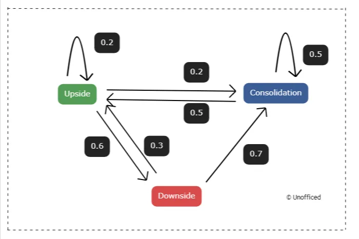
Hypothetical Markov Chain Exploration
This Markov Chain is an example model with random values as a probability which can be seen in the weighted arrows!
What is a Random Walk?
A random walk is a mathematical concept that describes a sequence of steps, each determined by random chance. In a Markov Chain, a random walk signifies a journey through different states, where the transition from one state to another is governed by certain probabilities.
The Markov Chain Connection
Markov Chains are characterized by the ‘memoryless’ property, meaning the probability of transitioning to the next state relies solely on the current state, not on the sequence of states that preceded it.
This characteristic lays the foundation for random walking within a Markov Chain.
In a financial context, let’s consider each state as a particular price level of a stock or an index. The random walk then symbolizes the daily price movements, where the transition probabilities represent the likelihood of price moving from one level to another.
Simulation for 1,00,000 Random Walks in a Markov Chain
Creating a simulation for 1,00,000 random walks in a Markov Chain requires a predefined transition matrix and an initial state.
The transition matrix contains the probabilities of moving from one state to another. Below is a simplified example to illustrate how you might set up such a simulation in Python using the numpy library:
					import numpy as np

# Assume a transition matrix (for simplicity, assuming a 3x3 matrix)
transition_matrix = np.array([
    [0.6, 0.3, 0.1],  # Transition probabilities from state 0 (Consolidation)
    [0.4, 0.4, 0.2],  # Transition probabilities from state 1 (Downside)
    [0.2, 0.5, 0.3]   # Transition probabilities from state 2 (Upside)
])

#This is an illustrative Purpose. You can also put the transition_matrix We derived in the last chapter.

# Initial state (assuming starting from Consolidation)
# This is not states_matrix.
current_state = 0  # 0: Consolidation, 1: Downside, 2: Upside

# Counters for the states
state_counts = {0: 0, 1: 0, 2: 0}

# Simulating 1,00,000 random walks
for _ in range(100000):
    next_state = np.random.choice([0, 1, 2], p=transition_matrix[current_state])
    state_counts[next_state] += 1
    current_state = next_state

# Calculating the frequency of each state
total_walks = sum(state_counts.values())
state_frequencies = {state: count/total_walks for state, count in state_counts.items()}

# Output the frequencies
print(state_frequencies)
In this code snippet:
- We first define a transition matrix that contains the probabilities of transitioning from one state to another.
- We initialize the current state to 0 (Consolidation) and create a dictionary to keep track of the count of each state.
- We then simulate 1,00,000 random walks using a for loop, where in each iteration, we use the numpy.random.choice function to randomly choose the next state based on the transition probabilities of the current state.
- We update the state count and the current state in each iteration.
- After the simulation, we calculate the frequency of each state by dividing the count of each state by the total number of walks and print the result.
- This code will output the frequency of each state after 1,00,000 random walks in the Markov Chain.
This exercise aimed to showcase the distribution of states over a large number of random sequences, further elucidating the concept of equilibrium or stationary distribution in a Markov Chain.
Here are the results of iterating this assumptive Markov Chain with 1,00,000 random walks –
					Downside         0.35191
Upside           0.21245
Consolidation    0.43564
Name: state, dtype: float64
So, we managed to find a Stationary State.
However, this method is not efficient as it doesn’t guarantee the discovery of all possible stationary states, particularly in Markov Chains with a large state space or complex transition dynamics.
We are just calling it “Stationary State” because it is derived from a large number of data points.
As We have already discussed earlier, In the context of Markov Chains, a Stationary State or Stationary Distribution is a probability distribution that remains unchanged in the Markov process over time.
Linear Algebra provides a more structured and mathematical approach to solving for the stationary distribution. Let’s find out.