Markov Chains in Stock Market Using Python – Getting Transition Matrix

Markov Chains in Stock Market Using Python - Getting Transition Matrix
In Our Last Chapter, We have discussed about Markov Chains with an example of Stock Market.
Now, we’ll delve into a more hands-on application by creating a Markov Chain using a sequence of “NIFTY 50” prices to model and predict future price behavior.
Getting the Sample Data
Let’s harness the power of Markov Chains to analyze a series of “NIFTY 50” prices with the aim of making informed predictions about future price movements.
So, first We shall use the NSEPython Library and use the index_history() function to get the last 100 trading days of data as a sample set. The NSEPython library is a tool designed to interface with publicly available data from the National Stock Exchange of India (NSE).
					from nsepython import *
symbol = "NIFTY 50"
days = 100
end_date = datetime.datetime.now().strftime("%d-%b-%Y")
end_date = str(end_date)

start_date = (datetime.datetime.now()- datetime.timedelta(days=days)).strftime("%d-%b-%Y")
start_date = str(start_date)

df=index_history("NIFTY 50",start_date,end_date)
print(df)
					#
	Index Name	INDEX_NAME	HistoricalDate	OPEN	HIGH	    LOW	        CLOSE
0	Nifty 50	NIFTY 50	02 Jul 2021	15705.85	15738.35	15635.95	15722.20
1	Nifty 50	NIFTY 50	01 Jul 2021	15755.05	15755.55	15667.05	15680.00
2	Nifty 50	NIFTY 50	30 Jun 2021	15776.90	15839.10	15708.75	15721.50
3	Nifty 50	NIFTY 50	29 Jun 2021	15807.50	15835.90	15724.05	15748.45
4	Nifty 50	NIFTY 50	28 Jun 2021	15915.35	15915.65	15792.15	15814.70
...	...	...	...	...	...	...	...
60	Nifty 50	NIFTY 50	05 Apr 2021	14837.70	14849.85	14459.50	14637.80
61	Nifty 50	NIFTY 50	01 Apr 2021	14798.40	14883.20	14692.45	14867.35
62	Nifty 50	NIFTY 50	31 Mar 2021	14811.85	14813.75	14670.25	14690.70
63	Nifty 50	NIFTY 50	30 Mar 2021	14628.50	14876.30	14617.60	14845.10
64	Nifty 50	NIFTY 50	26 Mar 2021	14506.30	14572.90	14414.25	14507.30
65 rows × 7 columns
The States of a Markov Chain
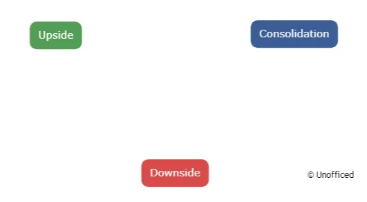
Building on the earlier discussion about applying Markov Chains to the NIFTY 50 index, we identified three distinct states that the index could exhibit on any given trading day:
- Upside: This state is observed when today’s price surpasses that of the previous day.
- Downside: This state occurs when today’s price is lower than yesterday’s.
- Consolidation: This is a state of price stability, where today’s price mirrors that of the previous day.
The first step in our analysis involves computing the daily returns from our dataset. This can be achieved by subtracting the previous day’s price from today’s price and dividing the result by the previous day’s price. The formula for daily return is given by:
Daily Return = (Today’s Price – Yesterday’s Price) / Yesterday’s Price
After calculating the daily returns, we need to create a function to categorize each day into one of the aforementioned states based on the daily return value.
However, a hurdle in characterizing the Consolidation state comes from the near impossibility of having an exact zero-price movement in real-world scenarios. The natural tendency of stock markets to react to various factors ensures that prices are almost always experiencing some level of change, however small.
To address this, we propose a modification to the definition of the Consolidation state to include minor price fluctuations within a specified range, rather than strictly zero movement. This range can be defined based on a threshold value or a percentage change that is considered negligible by the analyst.
Thus, the Consolidation state could be refined as follows:
Consolidation: The price movement is within a predefined small range, say between -0.5% and +0.5%, indicating a relatively stable price.
This adjustment aligns with the realistic dynamics of stock market prices and ensures a more accurate state classification in our Markov Chain model, setting a solid foundation for the subsequent stages of analysis.
					# Calculate the percentage change in closing prices
df["state"] = df["CLOSE"].astype(float).pct_change()

# Apply a function to classify each day based on the percentage change
df['state'] = df['state'].apply(
    lambda x: 'Upside' if (x > 0.001)  # If change is more than 0.1%, classify as 'Upside'
    else ('Downside' if (x <= 0.001)    # If change is 0.1% or less, classify as 'Downside'
    else 'Consolidation')               # If none of the above, classify as 'Consolidation'
)

# Display the last few rows of the dataframe
df.tail()
Output –
We are using the df.tail() function to limit the output to the last 5 rows to soothe the eyes.
					#
    Index Name	INDEX_NAME	HistoricalDate	OPEN	HIGH	    LOW	        CLOSE   	state
60	Nifty 50	NIFTY 50	05 Apr 2021	14837.70	14849.85	14459.50	14637.80	Downside
61	Nifty 50	NIFTY 50	01 Apr 2021	14798.40	14883.20	14692.45	14867.35	Upside
62	Nifty 50	NIFTY 50	31 Mar 2021	14811.85	14813.75	14670.25	14690.70	Downside
63	Nifty 50	NIFTY 50	30 Mar 2021	14628.50	14876.30	14617.60	14845.10	Upside
64	Nifty 50	NIFTY 50	26 Mar 2021	14506.30	14572.90	14414.25	14507.30	Downside
Now, the pct_change() the function of Pandas library is to show the prior day’s price to today’s price. That’s hence Today's State.
- But, We want to analyze the transitions from
Yesterday's StatetoToday's State. - That’s why, We are adding a new column
priorstatethat contains the values ofYesterday's State.
					# Shift the 'state' column down by one row to create a 'priorstate' column
df['priorstate'] = df['state'].shift(1)

# Display the last few rows of the dataframe
df.tail()
Output –
					#
    Index Name	INDEX_NAME	HistoricalDate	OPEN	HIGH	    LOW	        CLOSE   	state	    priorstate
60	Nifty 50	NIFTY 50	05 Apr 2021	14837.70	14849.85	14459.50	14637.80	Downside	Downside
61	Nifty 50	NIFTY 50	01 Apr 2021	14798.40	14883.20	14692.45	14867.35	Upside  	Downside
62	Nifty 50	NIFTY 50	31 Mar 2021	14811.85	14813.75	14670.25	14690.70	Downside	Upside
63	Nifty 50	NIFTY 50	30 Mar 2021	14628.50	14876.30	14617.60	14845.10	Upside  	Downside
64	Nifty 50	NIFTY 50	26 Mar 2021	14506.30	14572.90	14414.25	14507.30	Downside	Upside
Now that we have the Current State and Prior State, We need to build the Frequency Distribution Matrix.
A Frequency Distribution Matrix in the context of Markov Chains is a table that shows how frequently different state transitions occur in a dataset. It displays the number of times the system moves from one state to another. This matrix is essential in understanding the behavior of a Markov Chain, as it provides a clear representation of the transition probabilities between states based on historical data.
Coding Frequency Distribution Matrix for Markov Chain Model
Now Let’s use the historical data to calculate the transition probabilities between states. This involves analyzing how often the price moves from one state to another. Having established both the Current State and Prior State, the next step involves creating the Frequency Distribution Matrix.
This matrix is instrumental in understanding the frequency of transitions between states from one day to the next. The clarity of its definition can be enhanced by examining the outcome of the provided code.
					# Create a new DataFrame with only 'priorstate' and 'state' columns, dropping any rows with missing data
states = df [['priorstate','state']].dropna()

# Group the data by 'priorstate' and 'state', count occurrences of each combination, and reshape it into a matrix
states_matrix = states.groupby(['priorstate','state']).size().unstack().fillna(0)

# Print the resulting transition matrix
print(states_matrix)
Output –
					state       	Downside	Upside
priorstate
Consolidation	1.0	        0.0
Downside	    26.0    	14.0
Upside	        14.0    	9.0
●
This matrix reveals that there
were 26 instances where NIFTY was down, given that the previous day was also
down.
●
Alternatively, there was only 1
instance when NIFTY was down following a day in the consolidation state.
This is what the Frequency Distribution Matrix
does!
Understanding the Frequency Distribution Matrix:
The Frequency Distribution Matrix reflects the count, or frequency, of occurrences of states based on the prior state.
- It essentially captures the transition dynamics between different market states from one trading day to the next.
- This matrix serves as a foundational element for further analysis, aiding in the prediction of future states based on historical data.
One might loosely say Frequency Distribution Matrix is the candlestick of the Markov Chain.
The Frequency Distribution Matrix in Markov Chains provides a more statistical and quantitative analysis, emphasizing the probabilities of transitions between predefined states. Where, Candlestick Patterns in Price Action offer a more qualitative analysis, where visual interpretations of candlestick patterns are relied upon for making trading decisions.
Transition Matrix Formation:
The next step in our journey through Markov Chains is to organize the transition probabilities into what is known as a transition matrix. Each element in this matrix, denoted as P(ij), signifies the probability of transitioning from state i to state j.
Now, as we have calculated the Frequency Distribution Matrix earlier, it’s time to calculate the Transition Matrix. During our discussion on the basics of Markov Chain, we highlighted two key points:
- Each arrow represents a transition from one state to another.
- The sum of the probabilities of the outgoing arrows from any state equals 1.
These points are the essence of the Transition Matrix.
It’s beneficial to look at the output first as it will provide a clearer perspective to define it in layman’s terms. By applying a simple normalization function to the Frequency Distribution Matrix, we obtain the Transition Matrix.
					# Convert the frequency distribution matrix into a transition probability matrix
transition_matrix = states_matrix.apply(lambda x: x / float(x.sum()), axis=1)

# Print the resulting transition probability matrix
print(transition_matrix)
The states_matrix function essentially organizes and counts how often different state transitions occur, based on historical data.
In our example, it’s looking at the prior state of NIFTY and the current state, counting how many times NIFTY went from an upside to a downside, from a downside to an upside, and so on.
Output –
					state	        Downside	Upside
priorstate
Consolidation	1.000000	0.000000
Downside    	0.650000	0.350000
Upside      	0.608696	0.391304
The Transition Matrix shows the probability of the occurrence instead of the number of occurrences like the Frequency Distribution Matrix. You can also notice the sum of the weights are always 1 from priorstate to state. Like –
P(state="Downside"/priorstate="Downside") + P(state="Upside"/priorstate="Downside")
= 0.65 + 0.35
= 1
That’s why it is also called “Initial Probability Matrix”.
It’s noteworthy that there’s no current state of Consolidation, leading to a 3×2 matrix instead of a 3×3 matrix. In matrix computations, when all the values in a column are zero, the column can be omitted.
Now, before we dive into a Pythonic approach for building the Markov Chain, let’s explore the relationship between the matrix and the Markov Chain in more depth.
The Transition Matrix is crucial for getting to know how the Markov Chain behaves. It’s a table that shows us the chance of moving from one state to another. Each spot in the table gives us a straightforward view of how likely a certain change is.
This table is not only good for getting a sense of how things might change but also for making educated guesses about what might happen next. By looking at this table, we can get a sense of whether things are steady or if there are repeating patterns, which could hint at what might come in the future.
Difference between frequency distribution matrix and transition matrix:
- The Frequency Distribution Matrix tallies the number of times transitions between states occur, providing a count of occurrences.
- On the other hand, the Transition Matrix calculates the probability of moving from one state to another by normalizing these counts, offering a probabilistic perspective on state transitions.
Q. What does the word matrix mean?

No. It’s not the Movie!
A matrix is a rectangular array of numbers, symbols, or expressions arranged in rows and columns. In mathematics and related fields like computer science and engineering, matrices are used to perform a variety of operations and solve systems of equations.
They provide a structured way to represent and manipulate linear relationships and are essential tools in many areas including physics, statistics, machine learning, and finance.
- A matrix is a fundamental concept in linear algebra, a branch of mathematics. It is used to solve systems of linear equations and to perform operations such as rotation and scaling in graphics.
- In physics, especially in quantum mechanics, matrices are crucial in representing and analyzing complex systems. They help in describing the states and behaviors of quantum systems.
- In computer science, matrices are vital in various algorithms and data processing techniques. They are used to represent and manipulate data, especially in fields like computer graphics and machine learning.
- In machine learning, matrices are essential for handling large datasets, representing neural networks, and performing operations like filtering, transformation, and classification.