Application of Markov Chains in Stock Market

Application of Markov Chains in Stock Market
In Our Previous Chapters, We have discussed about Stochastic Modeling and Markov Model in Stock Market. We’ll begin our exploration with the simplest and most intuitive among these: the Markov Chain. A detailed examination of other Markov models will follow in subsequent discussions.
The States of a Markov Chain: An Example with the NIFTY Index
To understand how a Markov Chain operates, let’s consider the NIFTY stock index as an example. The NIFTY index, like any stock index, can exhibit different behaviors on any given day.
State Space
The entirety of all possible states a system can exist in is referred to as the state space.
Let’s consider the dynamics of the NIFTY index, which could exhibit three distinct states on the following day:
- Green (Positive Change): The index closes higher than its opening value.
- Red (Negative Change): The index closes lower than its opening value.
- Unchanged: The index closes at the same value as it opened.
State Frequency
- Each state is a unique occurrence or event within the system.
- The frequency of occurrence for a state is depicted by the number of arrows pointing to it in a state transition diagram, illustrating how often the market is likely to be in that state.
Utilizing the Markov Chain theory, we can establish a method to anticipate the state of the NIFTY index tomorrow, based on its state today. This theory provides a mathematical framework to model the transition probabilities between different states over time.
For instance, if NIFTY has been ending in green for a series of consecutive days, the Markov Chain theory can help quantify the probability of NIFTY ending in green, red, or remaining unchanged tomorrow.
Transition Probablity and Transition Matrix
This is done by calculating the transition probabilities based on historical data and today’s state.
Furthermore, these transition probabilities can be represented in a transition matrix, which provides a systematic way to model the likely transitions between states. This matrix is a fundamental component of the Markov Chain theory, enabling investors and analysts to forecast future states of the market, thus aiding in informed decision-making.
Example of a Markov Chain in Stock Market
Given that our system includes distinct states, exhibits randomness, and adheres to the Markov property—that the future state is conditional only on the current state—it’s appropriate to model our system as a Markov chain. Furthermore, our modeling will be conducted in discrete time intervals.
For example –
Tomorrow, there is 60% chance NIFTY’s state (By state in this context we mean NIFTY will close in) will be Upside given that today its state is Downside. We are using the term State because that is the convention.
Let’s say, there is a 20% chance that tomorrow, NIFTY’s state will be Upside again if today its state is Upside. You can see it is represented with a Self Pointing arrow.
We can depict this scenario using arrows in a diagram where the arrow starts from the current state (downward trend) and points towards the future state (upward trend). Let’s represent this in the diagram in weighted arrows. The arrow originates from the current state and points to the future state.
This is also called a Transition State Diagram. Since we have three states we will henceforth have a three-state Markov chain.
Each arrow is called a transition from one state to another. In the diagram here, You can see all the possible transitions. This diagram is called Markov Chain.
States: There are three primary states depicted in the diagram:
- Upside: Represented by a green rectangle “Upside”.
- Consolidation: Represented by a blue rectangle “Consolidation”.
- Downside: Represented by a red rectangle “Downside”.
Transitions & Probabilities:
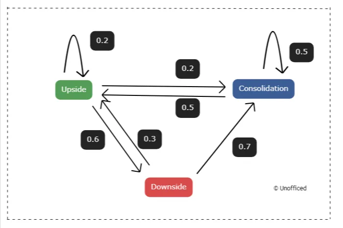
Transitions between states are indicated by arrows, and the probabilities of each transition are displayed as numbers adjacent to the arrows. Here’s a breakdown:
From Upside:
- To itself with a probability of 0.2 (depicted by an arrow looping back).
- To Consolidation with a probability of 0.2.
- To Downside with a probability of 0.6.
From Consolidation:
- To itself with a probability of 0.5 (depicted by an arrow looping back).
- To Upside with a probability of 0.5.
From Downside:
- To Consolidation with a probability of 0.3.
- To itself with a probability of 0.7 (depicted by an arrow looping back).
Here, you can observe all potential hypothetical transitions between the different states of the NIFTY index.
Let us encode it into a transition matrix P:
$$
P = \begin{bmatrix}
P_{11} & P_{12} & P_{13} \\
P_{21} & P_{22} & P_{23} \\
P_{31} & P_{32} & P_{33} \\
\end{bmatrix}
=
\begin{bmatrix}
0.2 & 0.2 & 0.6 \\
0.3 & 0.5 & 0.2 \\
0.5 & 0.7 & 0.5 \\
\end{bmatrix}
$$
Our Markov chain is now fully described by a state transition diagram and a transition matrix denoted by \( P \). The transition matrix \( P \) is fundamental to our model as it predicts future states, with the matrix’s powers indicating probabilities for multiple time steps ahead:
- \( P^2 \) forecasts the probabilities two time steps into the future.
- \( P^3 \) forecasts three time steps ahead, and so on.
This recursive multiplication of \( P \) outlines potential future outcomes of the Markov model.
- To project accurately, we must take into account the initial state vector \( q \), which represents the starting conditions such as bull, bear, or stagnant markets.
- For example, if we initiate in a bull market state, our \( q \) would be \( q = [1 \ 0 \ 0] \).
If we aim to predict the market condition two days forward, we are essentially calculating the probability distribution of the market states two steps ahead.
Now that We have known the basics of the Markov Chain, Let’s explore our Markov Chain doing in a more pythonic way in our next discussion.