Coin Tosses to Stock Trades: The Probability Connection

A coin is more than just a piece of currency; it’s a staple in the study of probability.
Used frequently to decide between two options, a coin’s design, featuring a head (H) and a tail (T), makes it an ideal candidate for random decision-making. Flipping a coin is essentially a probabilistic experiment with two possible outcomes, making it a classic case of binomial probability. A fair coin has an equal chance of landing on heads or tails, with each outcome holding a 50% probability.
For a single flip of a fair coin, the potential outcomes, or the sample space (S), are:
S = {H, T}
What about two flips?
S = {HH, HT, TH, TT}
Imagine flipping the coin 12 times:
H, T, T, H, H, H, T, H, T, T, H, T
Or 100 times:
H, T, T, H, H, H, T, H, T, T, H, T, … (continuing until the 100th flip).
Each outcome has an equal probability of 50%. If we denote the number of flips as N, this sequence comprises N discrete events. (“Discrete” refers to the nature of the events or outcomes being separate and distinct. Each flip of the coin is an individual event with its own outcome (heads or tails), not influenced by or blended with the outcomes of other flips. This term is used to emphasize that each coin flip is a standalone event, with a clear and separate result.)
A Coin Toss Game
Let’s consider a simple game where a coin flip determines your next move: heads, you step right; tails, you step left.
To track your position, we must first establish your starting point. This sets the origin, and since your movements are linear (left or right), they can be represented on the x-axis. We can then assign numerical values to the coin toss outcomes:
- Heads = +1
- Tails = -1
Repeating this process N times, we can represent your final position (D) as the sum of individual moves:
D = x1 + x2 + x3 + … + xN
An important question arises: what is the expected final position (E(D))?
Each coin toss (x) in a fair game has an expected value (E(x)) of zero:
E(x) = (-1 * 0.5) + (1 * 0.5) = 0
This indicates that the expected result for each step, whether it’s the first step (x1) or the final one (xN), is zero.
Therefore, we can infer that the expected overall outcome E(D) equals zero because it is the total of the expected results of each individual step, from the first to the last.

In simpler terms, if you were to track your position after many rounds of this game, you’d likely find yourself back at the starting point. On average, there’s no forward or backward progress. This kind of back-and-forth motion without a clear direction is known as a random walk.
Random Walks: A Pathway from Coin Flips to Stock Market Predictions
Part 1: Understanding Coin Toss Game and Stock Movements
Coin Toss Basics:
- A fair coin has two sides: heads (H) and tails (T).
- Each side has an equal chance of landing face up, which is a 50% probability, referred to as ‘p’.
Game Dynamics:
- In our game, flipping a coin decides if you move left or right.
- Heads means you take a step to the right (+1), and tails to the left (-1).
- After many flips, you’re expected to end up back where you started, which is the central point or ‘zero’ because the steps to the left and right cancel each other out.
Part 2: Adjusting the Model for Predictive Purposes
Introducing Drift:
- To potentially move away from the starting point, we adjust the probability ‘p’.
- If ‘p’ is set higher than 0.5, there’s a greater chance of moving to the right.
- Conversely, if ‘p’ is lower than 0.5, moving to the left becomes more likely.
Impact on Final Position:
- This adjustment to probability creates a ‘drift’ in one direction.
- The final position (D) is no longer expected to be zero but now has a bias towards the direction with the higher probability.
Stock Price Movement Analogy:
- By applying this model, we can simulate how a stock price might randomly fluctuate.
- Although stock prices do not move exactly as a coin flip, this random walk model gives us a basic framework to understand market movements.
- The key assumption here is that stock price changes have an element of randomness, similar to the coin toss game.
Part 3: Enhancing the Stock Movement Model
Moving Beyond the Basics:
- Rather than simply moving left or right, we’re now going to model the movement of a stock’s price.
- The starting point isn’t zero—it’s the actual stock price, and we’ll use the y-axis to track price changes over time.
Flexible Probability:
- We’ll let the probability ‘p’ vary, making it a random number between 0 and 1 for each move or time step.
- If ‘p’ is more than 0.5, it’s like getting heads, suggesting an increase in stock price.
- If ‘p’ is less than 0.5, it’s akin to tails, indicating a decrease in stock price.
Part 4: Introducing Proportionality and Geometric Walks
From Arithmetic to Geometric:
- Instead of fixed increases or decreases, we consider proportional changes, as stock prices change in percentages.
- This change turns our model from a straightforward arithmetic random walk into a geometric random walk.
Modeling Stock Price Changes:
- For a heads outcome, we increase the stock price by 1%.
- For tails, we decrease it by 1%.
- This process is repeated through ‘N’ iterations, simulating realistic stock price movements.
Practical Application:
- We’ll simulate the price movement of a well-known stock—using Infy as an example—with an initial price of 100 day’s before’s price of INFY
- Using computational tools, we model these changes over a set period, say 100 days, to see the path the stock price might take.
Here’s a Python code snippet using the nsepython package to simulate a similar process for an Indian stock:
					import numpy as np
import matplotlib.pyplot as plt
from nsepythonserver import *

# Define the stock symbol and get the starting price
# Define the symbol and series
symbol = "INFY"
series = "EQ"

# Calculate dates dynamically
end_date = datetime.datetime.now().strftime('%d-%m-%Y')  # Today's date
start_date = (datetime.datetime.now() - datetime.timedelta(days=100)).strftime('%d-%m-%Y')  # Date 100 days ago

# Fetch the historical equity data
historical_data = equity_history(symbol, series, start_date, end_date)

# historical_data would be a DataFrame containing the historical prices of INFY
starting_price = historical_data['CH_LAST_TRADED_PRICE'].iloc[-1]


# Define the number of days for the simulation
days = 100
prices = [starting_price]  # Starting price is the first item in our list of prices

# Simulate the geometric random walk
for _ in range(days):
    p = np.random.uniform(0, 1)  # Randomly select the probability p
    if p > 0.5:
        prices.append(prices[-1] * 1.01)  # Increase by 1% for 'heads'
    else:
        prices.append(prices[-1] * 0.99)  # Decrease by 1% for 'tails'

plt.figure(figsize=(14, 7))
plt.plot(prices, label='Simulated Stock Price')
plt.title(f"Simulated Stock Price Movement for {symbol} over {days} Days")
plt.xlabel('Day')
plt.ylabel('Price (INR)')
plt.legend()
plt.grid(True)
# Add the watermark text
plt.text(0.5, 0.5, 'unofficed.com', fontsize=40, color='gray', ha='center', va='center', alpha=0.5, transform=plt.gcf().transFigure)
plt.show()
To dynamically get the price of the stock symbol “INFY” from 100 days ago to today, you would first determine the current date, calculate the date 100 days ago, and then pass those dates to the equity_history function.
Anyways, The outcome i.e. the Graph of our geometric random walk model for Infosys Company stock over 100 days looks like –
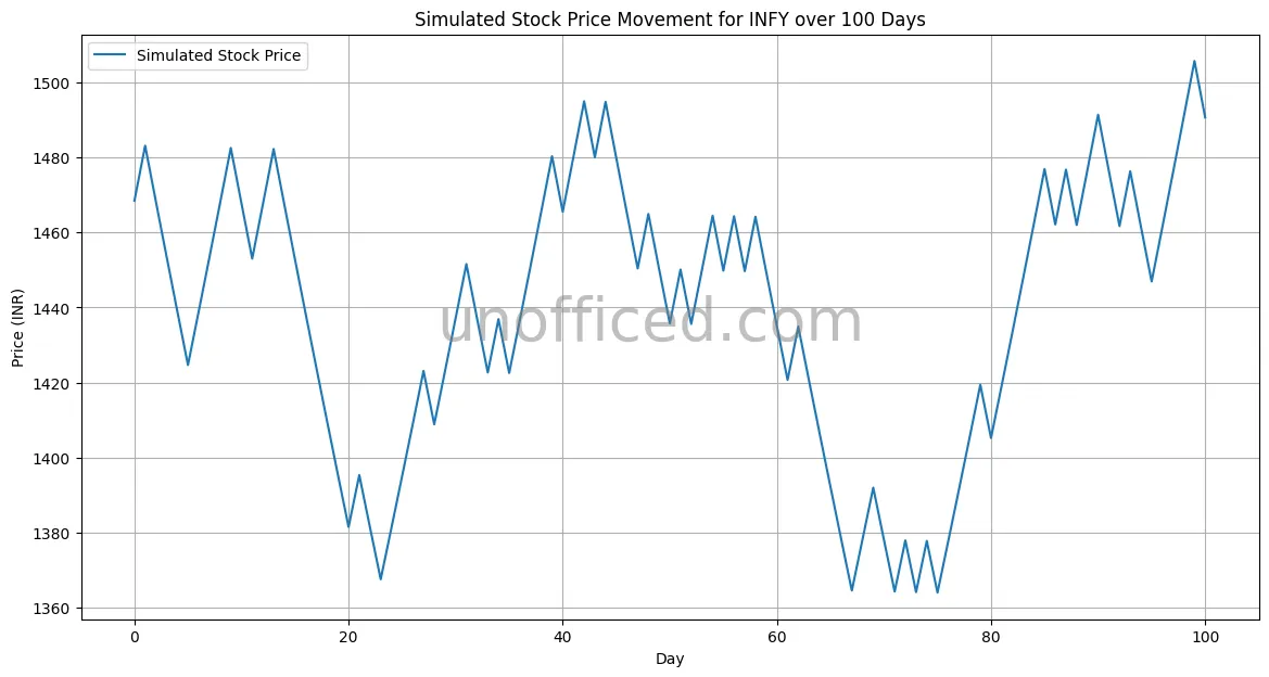
It’s quite remarkable, isn’t it? It’s fascinating to see the resemblance between the simulated and actual data, particularly how closely their final prices align after 100 days, being nearly identical!
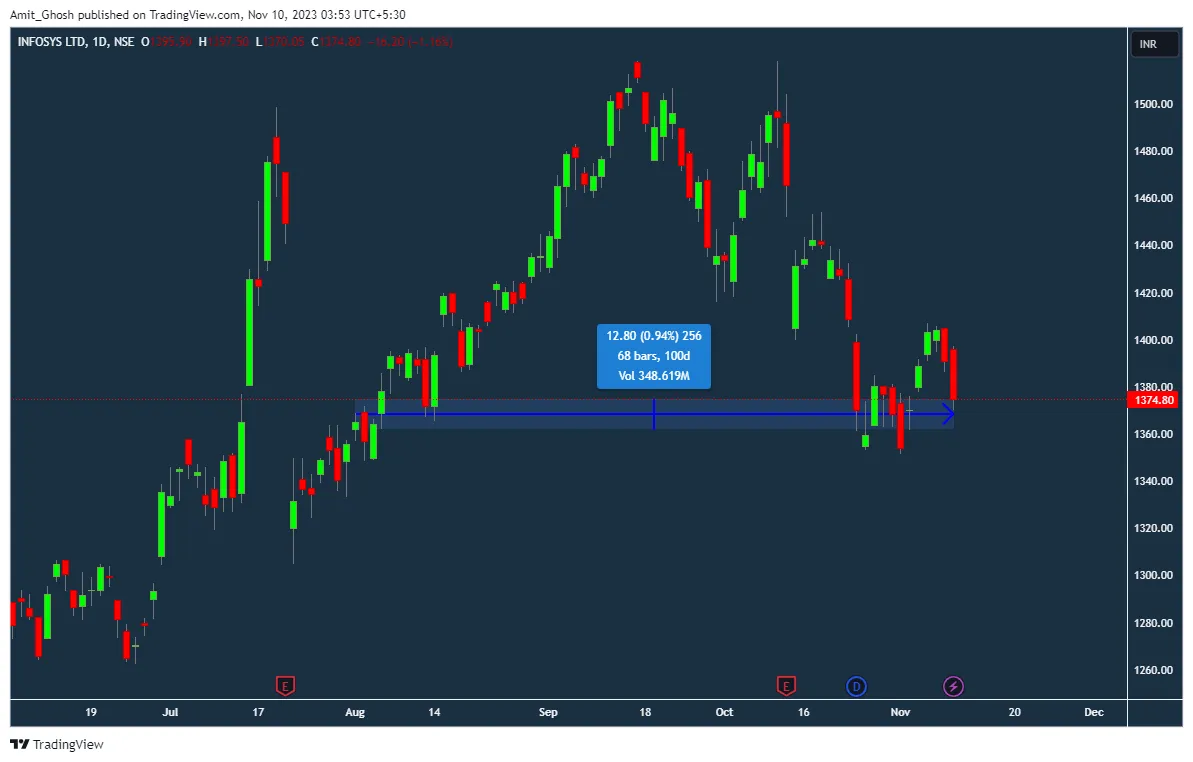
However, what’s truly notable is the similarity in the price trends — the patterns of the graphs are almost identical.
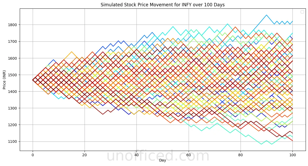
How about 100 Simulations?
When looking at the results, it’s key to remember that this might be a one-off case. The model used here is quite basic. However, it provides a foundation for beginning to understand how prices for various financial products can move. The use of mathematical and physical theories, like random walks leading to Brownian motion, is common in building models for financial markets.
How about we run the random walk simulation 100 times, each iteration displayed in a different color? Let’s take our old code snippet and deploy a loop over it.
					import numpy as np
import matplotlib.pyplot as plt
from nsepythonserver import *

# Define the stock symbol and get the starting price
# Define the symbol and series
symbol = "INFY"
series = "EQ"

# Calculate dates dynamically
end_date = datetime.datetime.now().strftime('%d-%m-%Y')  # Today's date
start_date = (datetime.datetime.now() - datetime.timedelta(days=100)).strftime('%d-%m-%Y')  # Date 100 days ago

# Fetch the historical equity data
historical_data = equity_history(symbol, series, start_date, end_date)

# historical_data would be a DataFrame containing the historical prices of INFY
starting_price = historical_data['CH_LAST_TRADED_PRICE'].iloc[-1]


# Define the number of days for the simulation
days = 100
prices = [starting_price]  # Starting price is the first item in our list of prices
forloops = 100  # Number of simulations to run

# Function to simulate geometric random walk
def simulate_geometric_random_walk(start_price, days):
    prices = [start_price]  # Starting price of the stock
    for _ in range(days):
        p = np.random.uniform(0, 1)  # Randomly select the probability p
        if p > 0.5:
            prices.append(prices[-1] * 1.01)  # Increase by 1% for 'heads'
        else:
            prices.append(prices[-1] * 0.99)  # Decrease by 1% for 'tails'
    return prices

plt.figure(figsize=(14, 7))
colors = plt.cm.jet(np.linspace(0, 1, forloops))  # Create a range of colors

# Run the simulation for the given number of forloops and plot them
for i in range(forloops):
    prices = simulate_geometric_random_walk(starting_price, days)
    plt.plot(prices, color=colors[i])

# Customize the plot
plt.title(f"Simulated Stock Price Movement for {symbol} over {days} Days")
plt.xlabel('Day')
plt.ylabel('Price (INR)')
plt.legend()
plt.grid(True)
# Add the watermark text
plt.text(0.5, 0.08, 'unofficed.com', fontsize=40, color='gray', ha='center', va='center', alpha=0.2, transform=plt.gcf().transFigure)
plt.show()
The output chart shows multiple paths of a simulated stock price over a set number of days, illustrating the concept of a geometric random walk. Each path represents a possible sequence of price changes, with the randomness reflecting the uncertainty inherent in stock price movements.
The key characteristics of this model in relation to the code are:
Multiplicative Factor: The stock price is multiplied by 1.01 if the random draw is greater than 0.5 (simulating a 1% increase) and by 0.99 if it’s not (simulating a 1% decrease). This multiplicative factor is what makes the process “geometric” as opposed to “arithmetic”.
Log-normal Distribution: Over many iterations, due to the multiplicative nature of the price changes, the final prices are expected to follow a log-normal distribution. This means that if you take the natural logarithm (ln) of the stock prices, the resulting values should be normally distributed.
Randomness: The randomness comes from the
np.random.uniform(0, 1)function which generates a uniformly distributed number between 0 and 1. This means every possible value within this range is equally likely to be chosen. The decision to increase or decrease the price is based on this random number.Terminal Prices: The final prices that you get after the last day of each simulation represent the terminal prices. If you were to run a very large number of simulations, the distribution of these terminal prices would become apparent. The shape of this distribution would be influenced by the random process defined in the code.
Upward Bias: While the direction of each individual simulation is unpredictable, the overall trend seems to be upward. This is due to the simulation rule that increases prices by 1% for ‘heads’ (which occurs when the random number is above 0.5) and decreases them by 1% for ‘tails’. Since the increase and decrease are not symmetrical (1% increase is not the same as 1% decrease), over many iterations, an upward bias is introduced.
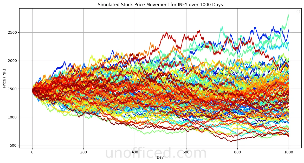
1000 Days!
Let’s be a mad man and do 1000 Days simulation. Thanks to our recent structured code, We just need to change one variable –
days = 1000
The output looks like this –