An Examination of the Wiener Process: Implications in Financial Analysis

In financial analysis and risk management, the Wiener Process or Brownian Motion holds significant relevance due to its capacity to model the randomness in the evolution of a variable over continuous time which is commonly observed in financial markets.
This process is fundamental to stochastic calculus, aiding in the analysis of complex financial instruments. This examination seeks to elucidate the Wiener Process and its substantial implications in risk management.
Core Attributes
The Wiener Process is a real-valued continuous-time stochastic process, which is characterized by four primary properties:
- Independence: Each increment is independent of others.
- Stationarity: The increments are stationary over time.
- Normality: The increments adhere to a normal distribution.
- Continuity: The process is continuous in time.
Historical Genesis
Brownian Motion was named after the botanist Robert Brown, who in the early 19th century, observed the erratic movement of pollen particles when suspended in water under a microscope.
This random motion, known as “Brownian Motion,” became a fundamental concept in the world of physics and was later used to provide empirical evidence of the existence of atoms.
It is characterized by a mean of zero and a variance that increases linearly with time (often standardized to one for each time interval), making it a standardized model for the random walk hypothesis.
While Brownian Motion was initially an observational phenomenon, the Wiener Process was its formal mathematical representation.
In the world of finance, these concepts lay the groundwork for understanding price movements and volatility in financial markets. Financial assets, especially stock prices, rarely move in a linear or predictable fashion. Instead, they exhibit properties that can be likened to the erratic movements Robert Brown observed.
Wiener Process
A Wiener process (often referred to as Brownian motion) is a continuous-time stochastic process that represents the integral of a white noise process. It’s named after Norbert Wiener. The main characteristics of a Wiener process are:
- \(W(0) = 0\): It starts at zero.
- The increments are independent: The change in the process over non-overlapping intervals of time are independent of each other.
- The increments are normally distributed: \(W(t + \Delta t) – W(t)\) is normally distributed with mean 0 and variance \(\Delta t\).
- It has continuous paths.
The Wiener process is often used in finance to model random movements in stock prices, and it forms the basis of the Black-Scholes option pricing model.
Python Code for Wiener Process:
					import numpy as np
import matplotlib.pyplot as plt

def simulate_wiener_process(num_points, dt):
    # Generate the increments using normal distribution
    increments = np.random.normal(0, np.sqrt(dt), num_points - 1)

    # The Wiener process starts at zero, so we concatenate a 0 at the beginning
    W = np.concatenate([[0], np.cumsum(increments)])

    return W

# Simulation parameters
num_points = 1000
dt = 0.01

W = simulate_wiener_process(num_points, dt)

# Plotting the Wiener process
plt.figure(figsize=(10, 6))
plt.plot(np.arange(num_points) * dt, W)
plt.title('Wiener Process')
plt.xlabel('Time')
plt.ylabel('W(t)')
plt.grid(True)
plt.show()
Numpy (np): This is a library in Python used for numerical calculations. It helps in doing complex math easily and is especially good at working with arrays (lists of numbers).
Matplotlib (plt): This is another library in Python used for creating graphs and charts. It helps in visually representing data, like drawing a line graph to show how something changes over time.
increments = np.random.normal(0, np.sqrt(dt), num_points – 1):
np.random.normal: Numpy function for generating random numbers.0: Mean of the normal distribution, centering the random numbers around 0.np.sqrt(dt): Standard deviation of the normal distribution, calculated as the square root ofdt.num_points - 1: The number of random numbers to generate, one less than the total points as the Wiener process starts at 0.
W = np.concatenate([[0], np.cumsum(increments)]):
np.concatenate: Numpy function to combine arrays.[[0]: Starting point of the Wiener process at 0.np.cumsum(increments): Calculates the cumulative sum of the increments, adding each random number to the sum of all previous numbers.- Concatenates
[0]with the cumulative sum to construct the entire Wiener process.
Output
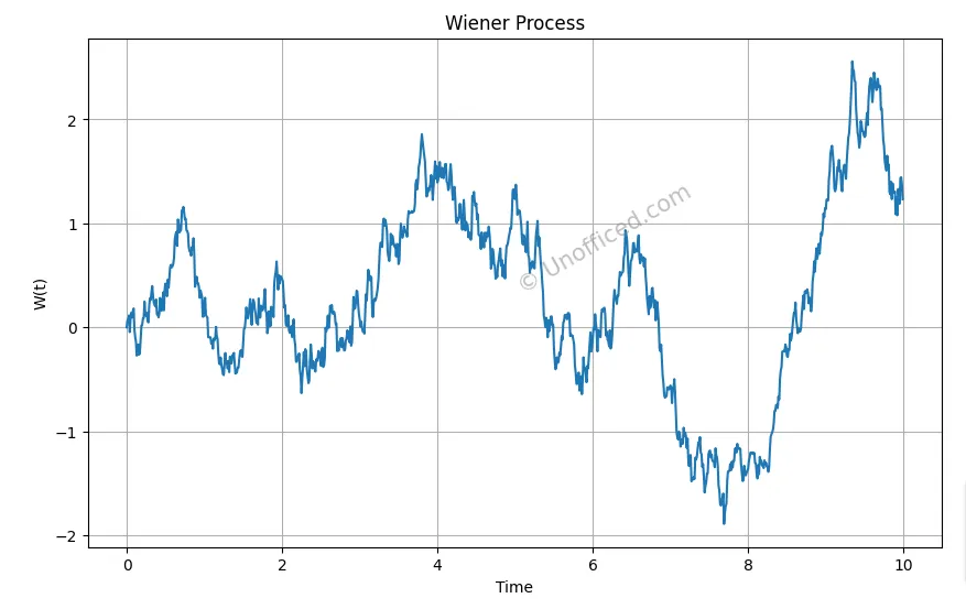
This code simulates and plots a single path of a Wiener process over a period defined by num_points and dt.
The increments over each interval dt are drawn from a normal distribution with a mean of 0 and a variance dt, and then they’re cumulatively summed to get the values of the Wiener process at each point in time.
Applications of the Wiener Process in Finance
Option Pricing in The Black-Scholes Model
The Black-Scholes Model, a groundbreaking formula for option pricing, relies heavily on the principles of Brownian Motion. Here’s why: An option’s value is derived from an underlying asset, typically a stock.
The future price of this stock is uncertain and can be thought of as moving randomly—much like a pollen particle suspended in water.
The Wiener Process, with its mathematical rigor, provides the necessary foundation to model this randomness in a way that’s suitable for financial calculations.
Apart from that, Here is an outline the various applications of the Wiener Process in financial analysis and risk management.
Risk Management: The Wiener Process is instrumental in risk management by offering a structured approach to model asset price dynamics. By quantifying the stochastic behavior of asset prices, risk managers can devise robust risk mitigation strategies and asset allocation frameworks, ensuring the resilience of financial portfolios against market volatility.Asset Price Forecasting: Underpinning the random walk hypothesis, the Wiener Process aids in modeling asset price dynamics. By recognizing the stochastic nature of asset prices, financial analysts can develop nuanced forecasting models, enhancing the accuracy and reliability of market predictions.
Portfolio Optimization: Incorporating the Wiener Process in portfolio optimization helps in understanding the probable price paths of constituent assets. This understanding is vital for optimizing asset allocation, managing portfolio risk, and ultimately enhancing portfolio performance over time.