How to Simulate Geometric Brownian Motion in a Stock

Stock prices are often unpredictable, affected by a myriad of factors from global events to company performance. However, for the sake of quantitative analysis, we can use mathematical models to simulate potential stock price movements. One of the most popular models for this purpose is the Geometric Brownian Motion (GBM).
To simulate the GBM for a stock, we’ll require:
- Initial stock price, \(S(0)\)
- Drift (\(\mu\)), typically the average daily return of the stock over a period
- Volatility (\(\sigma\)), usually the standard deviation of the daily return over a period
In our example, we’ll fetch the daily drift and volatility from historical stock prices using Python and the nsepython package, which provides data for Indian stock markets.
Step 1: Fetching Drift and Volatility
Using the nsepython package, we can define functions to fetch the daily drift and volatility for a given stock:
					from nsepython import *

def get_daily_drift(symbol, series, start_date, end_date):
    historical_data = equity_history(symbol, series, start_date, end_date)
    daily_returns = historical_data['CH_CLOSING_PRICE'].pct_change().dropna()
    daily_drift = daily_returns.mean()
    return daily_drift

def get_daily_volatility(symbol, series, start_date, end_date):
    historical_data = equity_history(symbol, series, start_date, end_date)
    daily_returns = historical_data['CH_CLOSING_PRICE'].pct_change().dropna()
    daily_volatility = daily_returns.std()
    return daily_volatility
Step 2: Simulating the GBM
With the drift and volatility values, we can now simulate the stock prices using GBM:
					import numpy as np

def simulate_gbm(S0, mu, sigma, dt, num_days, num_simulations):
    stock_price_paths = np.zeros((num_days, num_simulations))
    stock_price_paths[0] = S0

    for t in range(1, num_days):
        rand_nums = np.random.randn(num_simulations)
        stock_price_paths[t] = stock_price_paths[t - 1] * np.exp((mu - 0.5 * sigma**2) * dt + sigma * np.sqrt(dt) * rand_nums)

    return stock_price_paths
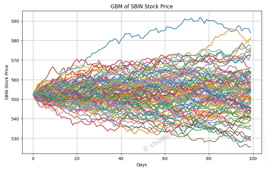
Step 3: Visualization
Visualizing the simulated paths gives an intuitive understanding of potential stock price movements:
					import matplotlib.pyplot as plt

# Parameters (e.g., for SBIN stock)
S0 = 552.4
mu = get_daily_drift("SBIN", "EQ", "01-01-2021", "31-12-2021")
sigma = get_daily_volatility("SBIN", "EQ", "01-01-2021", "31-12-2021")
dt = 1/252
num_days = 100
num_simulations = 10000

stock_price_paths = simulate_gbm(S0, mu, sigma, dt, num_days, num_simulations)

plt.figure(figsize=(10,6))
plt.plot(stock_price_paths[:, :100])
plt.title('GBM of SBIN Stock Price')
plt.xlabel('Days')
plt.ylabel('SBIN Stock Price')
plt.grid(True)
plt.show()
Output:
Geometric Brownian Motion provides a simplistic yet powerful model to understand and visualize the unpredictability of stock prices.
While the model has its limitations and assumptions, it’s a great starting point for quantitative finance enthusiasts and professionals to delve deeper into the world of financial modeling. Always remember to base your simulations on reliable data and adjust the parameters according to the stock and market in question.