Markov Chain and Linear Algebra – Calculation of Stationary Distribution using Python

“The stock market is like a game of chess, but with the added thrill of a roller coaster. And the roller coaster is on fire.”
—Artem Kalashnikov
In Our Last Chapter, We have discussed about Random Walk in Markov Chain using python. Now, We shall dive into more detail into Markov Chain and its relation with linear algebra more theoretically.
Representing Markov Chain Using Linear Algebra
In tackling this model, we’ll employ Linear Algebra. Given that we’re dealing with a directed graph, it can be conveniently represented using an Adjacency Matrix.
If you’re unfamiliar with the term, we’ve previously encountered the use of an adjacency matrix in our last discussion where we designed a Transition Matrix utilizing Pandas.
So, the Markov Chain above will translate into –
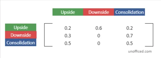
An adjacency matrix is a square grid used to show a graph’s structure.
- In our case, it helps show the transitions between different states in a Markov Chain.
- Each spot in the matrix tells us the chance of moving from one state to another.
This matrix makes it easier to understand and work with Markov Chains.
The Transition Matrix
In our journey through understanding Markov Chains, we come across a crucial component known as the Transition Matrix. This matrix plays a fundamental role in encapsulating the dynamics of state transitions within the chain.
Let’s dive a little deeper to understand its structure and significance.

Matrix Elements Representing Transition Probabilities:
- The elements within the Transition Matrix aren’t mere numbers; they hold the essence of the probabilistic transitions between states in a Markov Chain.
- For instance, the element located at the intersection of the second row and the first column encapsulates the transition probability from a Downside state to an Upside state. This numerical value represents the likelihood of this particular state transition.
Zero Elements Indicating Absence of Transition:
A zero value within the matrix isn’t arbitrary; it holds meaning. A zero element indicates that there’s no transition possible between the corresponding states. In graphical terms, it means there’s no edge connecting these two vertices (states) in the directed graph representing the Markov Chain.
Naming and Notation:
This significant matrix is termed the “Transition Matrix,” often denoted by the symbol ‘A’ for ease of reference in mathematical discussions and computations.
Transition Matrix as a Gateway to State Dynamics:
- The Transition Matrix isn’t just a static representation; it’s a gateway to understanding the dynamics of state transitions.
- Through it, we can dive into the probable future states given the current state, providing a foundation for forecasting and analysis in various applications, including finance, where Markov Chains find substantial utility.
The Transition Matrix, in essence, forms the backbone of the Markov Chain, providing a structured, numerical way to explore, analyze, and predict state transitions within the chain. As we move forward, we’ll see how this matrix, denoted as ‘A’.
Forecasting Futures Probabilities of States
Remember that, Our goal is to find the probabilities of each state.
State Probabilities:
- Initially, you’re considering a scenario where the market is in a ‘Downside’ state on the first day (t=0).
- The probabilities of being in each state are represented by a row vector π. In this scenario, π_0 = [0 1 0] signifies that the probability of being in the ‘Downside’ state is 1 (or 100%), while the probabilities of being in the ‘Upside’ and ‘Consolidation’ states are 0 (or 0%).
A row vector is a type of matrix with a single row and multiple columns. Each element in this row corresponds to a value associated with a particular column. In mathematical notation, it’s often represented as a horizontal array of numbers.
So π will look like – π_0 = [ 0 1 0 ]
- The second element which corresponds to the Downside state becomes 1.
- And, the other two remain 0.
Matrix Multiplication:
Now, Let’s see what happens if we multiply our row vector with the transition matrix. When you multiply the row vector π_0 by the Transition Matrix A (i.e., π_0.A), you’re essentially calculating the probabilities of transitioning to each future state from the current ‘Downside’ state.
The Initial Transition Matrix
Future Probabilities corresponds to the Downside State
The Initial Transition Matrix
Future Probabilities corresponding to the Downside state.

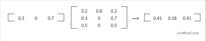
So, π_0.A =

The result of the multiplication gives you the second row of the Transition Matrix. Do note that We are not diving deep into the formulas of matrix multiplication.
This multiplication results in a new row vector which gives the probabilities of being in each state in the next time step (t=1), based on the current state being ‘Downside’.
This row corresponds to the ‘Downside’ state, and each element in this row now represents the probability of transitioning from the ‘Downside’ state to each of the three possible states (‘Upside’, ‘Downside’, ‘Consolidation’) in the next time step.
- In essence, by performing this multiplication, you’ve moved one step forward in time, and now have a new set of probabilities for the states at t=1 based on the current state at t=0.
- The resulting row vector from the multiplication provides the future probabilities corresponding to the ‘Downside’ state.
- It’s a snapshot of how likely the market is to transition to each state in the next time step, given the current state.
Construction of the Markov Chain
This process can be continued to calculate state probabilities for further time steps by repeatedly multiplying the resulting row vector with the Transition Matrix. In this step, Let’s iterate the Markov Chain forward in time by continually multiplying the current state probability vector (π) with the transition matrix (A). Then, We keep extending it –
Initially, we have π_0 (the state probabilities at time t=0).
By multiplying π_0 with A, we obtain π_1, which represents the state probabilities at time t=1.
So, π_1.A =
Similarly, π_2.A =
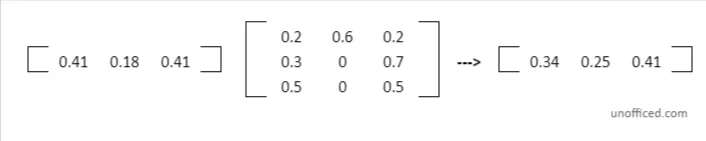
This process is repeated to move forward through time steps: π_1.A = π_2, π_2.A = π_3, and so on. Each multiplication gives us the state probabilities for the next time step.
This process of multiplying the state probability vector with the Transition Matrix to obtain future state probabilities is a core aspect of working with Markov Chains. It demonstrates how the chain evolves over time and how the probabilities of being in each state change with each time step, based on the current state and the transition probabilities defined in the Transition Matrix.
Eigenvector Equation and Markov Chain
Objective: The primary goal when working with Markov Chains is to find a stationary state. A stationary state is a state where the probabilities no longer change with further transitions.
A stationary state, represented as π, would satisfy the equation π.A = π. This means that when you multiply this state vector by the transition matrix (A), the result is the same state vector.
Connecting to Eigenvector Equation:
An eigenvector of a square matrix A is a nonzero vector x such that when A operates on x, the result is a scalar multiple of x. This relationship is expressed by the eigenvector equation: Ax = λx where:
- A is a square matrix,
- x is a vector (not the zero vector),
- λ is a scalar known as the eigenvalue associated with the eigenvector x.
The equation π.A = π is analogous to the eigenvector equation Ax = λx from linear algebra. In this equation:
- A is a matrix
- x is an eigenvector of A
- λ is the eigenvalue corresponding to that eigenvector
In the context of Markov Chains, we’re specifically looking for an eigenvector π where the eigenvalue λ is 1. This is because the stationary state vector remains unchanged when multiplied by the transition matrix.
Finding the Stationary State:
Besides being an eigenvector with eigenvalue 1, the elements of π must sum to 1 because they represent a probability distribution across states.
This results in two equations:
- π.A = π (Equation 1 = Equation representing the stationary state) and
- Sum of all elements of π = π[1] + π[2] + π[3] = 1 (Equation 2 = Equation ensuring the probabilities sum up to 1).
These equations together aid in finding the stationary state π.
Once π is found, it provides the equilibrium or stationary distribution of the Markov Chain, which remains unchanged upon further transitions.
By employing linear algebra concepts, particularly eigenvectors and eigenvalues, we can solve for the stationary distribution π of the Markov Chain in a more efficient and theoretical manner. This approach provides an elegant way to understand and calculate the long-term behavior of the Markov Chain, bridging probabilistic models with linear algebraic theory.
Calculation of Eigenvector (π) of the Hypothetical Model
From π.A = π
We get three equations from here –
0.2x + 0.3y + 0.5z = x0.6x = y0.2x + 0.7y + 0.5z = z
From: π[1] + π[2] + π[3] = 1
We get one equation from here –
x + y + z = 1
After solving,
π = [25/71, 15/71, 31/71] = [0.35211, 0.21127. 0.43662]
In the last discussion, We calculated the value of π using the Random Walk Theory.
It was –
π = [0.35191,0.21245,0.43564]
Verification through Random Walk:
Previously, using the Random Walk theory, a similar vector π was derived:
π = [0.35191,0.21245,0.43564]
The close similarity between the π values obtained by both methods validates the consistency and robustness of the Markov Chain model.
The alignment of results from two distinct methods – one theoretical (linear algebra) and one empirical (random walk) – showcases the utility and reliability of Markov Chains in analyzing stochastic processes.
This comparison also illustrates how linear algebra provides a more structured and analytical way to find the stationary distribution, which is a crucial aspect in understanding the long-term behavior of Markov Chains.
Multiple Stationary States
It’s possible for a Markov Chain to have more than one stationary state. This occurs if there are multiple eigenvectors corresponding to the eigenvalue of 1 in the transition matrix. Each of these eigenvectors represents a different stationary state.
Limitation of Random Walk Method:
The random walk method discussed earlier could miss some of these stationary states because it essentially simulates the evolution of the Markov Chain from a specific starting point.
If there are multiple stationary states, the random walk method might only converge to one of them, based on the starting state and the structure of the transition matrix.
Advantages of Linear Algebraic Approach:
By employing linear algebra, specifically by solving for eigenvectors of the transition matrix with an eigenvalue of 1, you can potentially uncover all stationary states that exist.
- This is because the algebraic method doesn’t depend on a particular starting state or a simulated process.
- It directly solves for states that satisfy the stationary condition (π.A = π).
Let’s jump back to our discussion using Python, connect the dots, and visually and numerically validate these concepts. This will solidify the understanding and ability to apply Markov Chains in practical scenarios