Backtest Entropy Alpha Bollinger Band Strategy Using Python with Equities Data

Let’s jump directly to the discussion from where we had left in the last part. So far We have checked out the trade performance and, analyzed that details with various popular trading metrics to get an overview of strength of our strategy.
In this part, We will apply the same in Equities data.
The Core Differences
- In Equity, We do not have different
instrument_tokenfor different expiry. So, We can backtest the entire dataset! - The code of getting the
priceof the stock andhighof the stock has to be changed and modified to get the equity data instead of derivatives data.
					#Price At The Particular Time

import datetime

# Your code here

# Create a function to get the price and high of a stock at a specific time
def get_stock_data(symbol, time):

    # Define the start and end date
    start_date = pd.Timestamp(time)
    end_date = start_date + datetime.timedelta(minutes=5)

    # Convert start and end date to string format
    from_date = start_date.strftime('%Y-%m-%d %H:%M:%S')


    # Fetch historical data for the stock
    data = kite.historical_data(instrument_token=get_insToken(symbol,"NSE"),
                                 from_date=from_date,
                                 to_date=from_date,
                                 interval='minute')

    # Return the price and high of the stock at that time
    return data[0]['open']


# Add new columns to the DataFrame
df['price'] = ''

# Iterate over each row of the DataFrame
for index, row in df.iterrows():
    # Get the stock symbol and triggered time
    symbol = row['Stocks (new stocks are highlighted)']
    time = row['Triggered at']

    # Get the price and high of the stock at the triggered time
    price= get_stock_data(symbol, time)

    # Update the price and high columns
    df.at[index, 'price'] = price
Rewriting the code to get the high of the equity price when we entered the trade –
					def get_high_of_day(kite, df):
    high_list = []
    for i, row in df.iterrows():
        # Get historical data for the trigger date of the stock
        symbol = row['Stocks (new stocks are highlighted)']
        data = kite.historical_data(instrument_token=get_insToken(symbol,"NSE"),
                                     from_date=row['Trigger Date'],
                                     to_date=row['Trigger Date'],
                                     interval='day')


        # Get the high of the day
        high = data[0]['high']
        high_list.append(high)

    df['high'] = high_list
    return df

df=get_high_of_day(kite, df)
df
Rewriting the code to simulate the trades in equity pricing system –
The Quant and Position Sizing
500000. It means if the stock price is 1381, it will short rounddown(500000/1381) = 362 quantity.
					import datetime


def find_day_high_time(kite, df):

    square_off_time_list=[]
    square_off_price_list=[]
    is_target_list = []

    for i, row in df.iterrows():

        # Get historical data for the trigger date of the stock
        symbol = row['stocks']
        data = kite.historical_data(instrument_token=get_insToken(symbol,"NSE"),
                                     from_date=row['Triggered at'],
                                     to_date=row['Triggered at'] + datetime.timedelta(days=1),
                                     interval='minute')

        is_target = False
        for i in range(0,len(data)):
            if(row["high"]==data[i]["high"]):
                is_target =True
                print("Target Triggered")
                #df.at[i, "is_target"] = True
                square_off_time_list.append(data[i]["date"])
                square_off_price_list.append(data[i]["high"])
                break

        if not (is_target):
            print("Target did not Trigger")
            square_off_time_var = datetime.datetime.strptime(str(row['Trigger Date'])+ " 14:50:00+05:30", '%Y-%m-%d %H:%M:%S%z')

            data1 = kite.historical_data(instrument_token=get_insToken(symbol,"NSE"),
                                     from_date=square_off_time_var,
                                     to_date=square_off_time_var,
                                     interval='minute')

            #print(data1)
            square_off_time_list.append(square_off_time_var)
            square_off_price_list.append(data1[0]["open"])

        is_target_list.append(is_target)


    df['square_off_time'] = square_off_time_list
    df['square_off_price'] = square_off_price_list
    df['is_target'] = is_target_list
    return df

df=find_day_high_time(kite, df)
df
					import math
quant_size = 500000

df["lotsize"] = df["price"].apply(lambda x: math.floor(quant_size/x))
df
The Final Trade Log
The above changes done in our old patch of code leads to this Final Trade Log –
					Triggered at	stocks	entry_price	high	square_off_time	square_off_price	is_target	lotsize	pl_points	pl
779	2022-09-13 10:01:00	HEROMOTOCO	2888.1	2903.00	2022-09-13 14:50:00	2865.00	False	173	-23.1	-3996.3
778	2022-09-13 10:01:00	DRREDDY	4284.85	4306.95	2022-09-13 14:50:00	4250.00	False	116	-34.85	-4042.6
775	2022-09-13 10:03:00	DIXON	4623.25	4670.00	2022-09-13 14:50:00	4605.05	False	108	-18.2	-1965.6
770	2022-09-13 10:06:00	ITC	331.7	335.00	2022-09-13 12:56:00	335.00	True	1507	3.3	4973.1
771	2022-09-13 10:06:00	SBICARD	957.4	961.00	2022-09-13 10:22:00	961.00	True	522	3.6	1879.2
...	...	...	...	...	...	...	...	...	...	...
5	2023-04-20 10:02:00	ICICIBANK	894.95	899.30	2023-04-20 14:50:00	893.85	False	558	-1.1	-613.8
4	2023-04-20 12:49:00	CUB	132.3	133.90	2023-04-20 15:16:00	133.90	True	3779	1.6	6046.4
3	2023-04-20 14:16:00	BAJAJ-AUTO	4311.1	4330.50	2023-04-20 14:50:00	4313.00	False	115	1.9	218.5
1	2023-04-21 09:58:00	ASIANPAINT	2853	2887.00	2023-04-21 14:23:00	2887.00	True	175	34.0	5950.0
0	2023-04-21 10:07:00	APOLLOTYRE	335.4	337.40	2023-04-21 14:50:00	333.95	False	1490	-1.45	-2160.5
477 rows × 10 columns
We have nearly 477 trades compared to 60 trades of last time giving a broader dataset spanning over half a year.
Calculate Trading Metrics
We can use the same patch of code used in the previous chapter to analyze the Trading Metrics. The column names of the database are also same. Anyways, The Output shows all the available info you need to know to evaluate a strategy –
Net P&L: 691606.25
Number of total trades: 477
Number of times target is hit: 187
Number of times stop loss is hit: 290
Win Ratio: 0.61
Avg PL: 1449.91
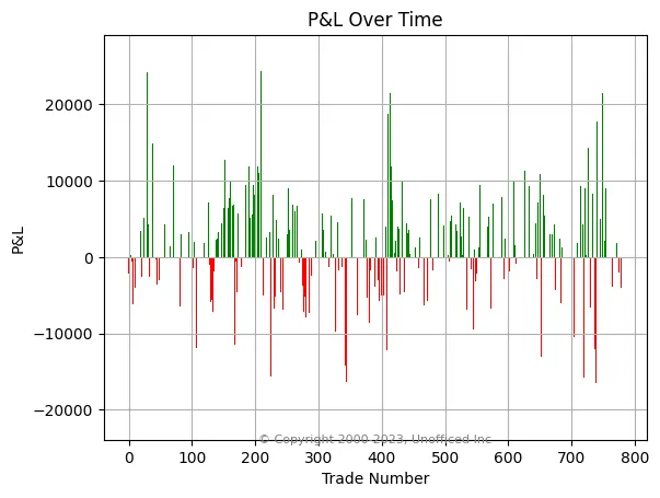
Max PL: 26645.0
Min PL: -21498.75
Gross P&L: 691606.25
Average Gain: 6019.51
Average Loss: -4897.87
Profit Factor: 0.58
Expected Payoff: 1449.91
Maximum Drawdown: 120861.8
Sharpe Ratio: 0.21
Gross Profit: 1661385.15
Gross Loss: -969778.9
Recovery Factor: 1.71
Maximum consecutive wins: 9
Maximum consecutive losses: 0
Maximal consecutive profit: 43535.70
Maximal consecutive loss: 30436.85
Average holding time: 0 days 05:08:35.345911949
Average holding time for profit trades: 0 days 05:34:04.130434782
Average holding time for loss trades: 0 days 04:35:01.212121212
Calculate the Profit/Loss over the Time
We can use the same code with matplotlib library to plot the graph. The graph looks like –
Plot the Cumulative Profit/Loss Over Time
We can use the same code from the last chapter to generate the graph – 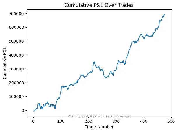
That concludes this discussion.