Probability of Profit

Usually, the Probability of Profit or, POP of an option trade means the chance of making at least 0.01 INR in that option trade (In other words, Not making loss!). It is roughly calculated using the greek Delta.
If you buy or sell an ATM option that has a delta of around 50, the probability of the option expiring in-the-money (ITM) or out-of-the-money (OTM) respectively is 50%, i.e. the trade has a success of 50% of being profitable at expiry.
Similar probability calculations are also done for the OTM options.
For an option buyer, a far OTM call/put option with a delta of 16 has a 16% probability of expiring ITM and profitable or 84% (100-16) chance of expiring OTM and worthless at expiry. For an options seller, it is 84% chance of making profit.
Also, We shall be calculating the POP with respect to the entire position i.e. we need to make sure delta reflects the lot size too while calculating.
It’s easy to calculate POP for naked puts or calls but gets a little complicated when calculating it for multi-legged strategies like strangle, straddle, ratio spreads, jade lizard etc.
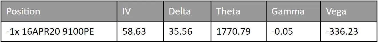
What is the POP of the option seller who sells 1 lot 9100PE?
100-35.56 = 64.44%
But, if we sell 2 lot 9100PE, the delta becomes 71.12. What is the POP?
It stays the same obviously! The probability does not change if you increase the amount in the position. To calculate POP, We need to consider 1 lot only. But as said, it becomes complex with more advanced strategies.
Linear Relationship
Just for clarification, delta and probability of expiring in the money are not the same thing. What we meant is that delta is usually a close enough approximation to the probability.
One way to think about it is to look at the probabilities and deltas of In the Money, Out of the Money, and At the Money options.
- A deep in the money option has a really high chance of expiring in the money, around 100%, and it has about 100 delta
- A far out of the money option has a really low chance of expiring in the money, around 0%, and it has about 0 delta
- An at the money option has about 50% probability of being in the money because there is a 50-50 chance the stock will go up or down, and it has about 50 delta
In these cases, the delta and probabilities are about the same. In fact if you look at an options chain with delta and probabilities, you can see that they are all about the same. In other words, there is a linear relationship between delta and probability.
Also note that – Delta varies as implied volatility changes. So does our POP.
Here is an example of increasing complexity of POP calculation. Let’s calculate the POP of an ATM short straddle. Before we dive into more details, we need to discuss two important concepts of mathematics.
Bayes Theorem
Bayes’ Theorem is a way of finding a probability when we know certain other probabilities.
The formula is:

It tells us how often A happens given that B happens, written P(A|B).
When we know:
- How often B happens given that A happens, written P(B|A)
- And how likely A is on its own, written P(A)
- And how likely B is on its own, written P(B)
Probability of Independent Events
But, Let’s say, there is no connection between two events.
P(A|B) = P(A).
P(B|A) = P(B).
- The probability of A, given that B has happened, is the same as the probability of A.
- Likewise, the probability of B, given that A has happened, is the same as the probability of B.
This shouldn’t be a surprise, as one event doesn’t affect the other.
So, there are two cases –
- When two events, A and B, are independent, the Probability of both occurring is P(A and B) = P(A) * P(B).
- When two events, A and B, are independent, the Probability of one of them occurring is P(A or B) = P(A) + P(B)
Probability of Profit for Straddles
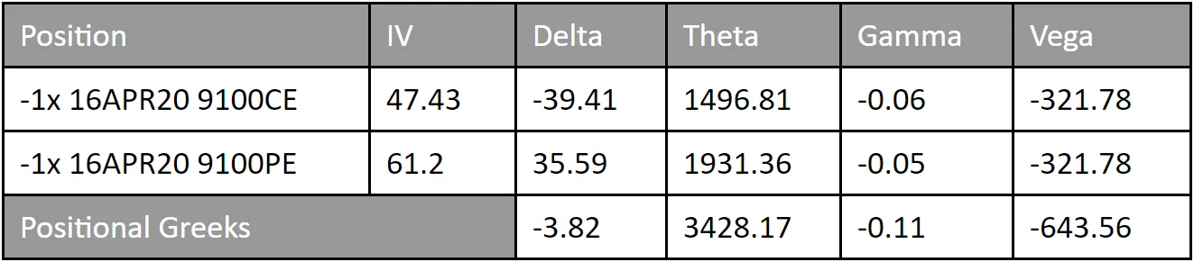
Right now, NIFTY’s LTP is 9111.9. Let’s say we have sold 9100PE and 9100CE of 16th Apr expiry to form a short straddle setup. The call options lower the breakeven of downside while the put options lower the breakeven of upside. Hence, POP of this setup is dependent on each other.
Current Setup –
- Sell NIFTY 16th Apr 9100PE at 213
- Sell NIFTY 16th Apr 9100CE at 253.7
To calculate POP, The correct approach is to find the Breakevens of this setup. In this case –
- Lower Breakeven: 9100 – (213 + 253.7) = 8633.3
- Upper Breakeven: 9100 + (213 + 253.7) = 9566.7
As we notice, Chances of breaking Lower Breakeven and Upper Breakeven are independent events! And, in a similar manner, We can calculate the POP of our breakeven breaking.
We can restructure the question as follows –
- What is the POP of 8650PE?
- What is the POP of 9550CE?
We need to take the nearest ITMs with respect to the Breakeven points.
- Delta of 8650PE is 23.32
- Delta of 9550CE is 21.63
So,
- Probability of Profit if we buy 8650PE is 23.32% or .2332
- Probability of Profit if we buy 9550CE is 21.63% or .2163
Now, if one of our breakeven breaks i.e. if one of 8650PE and 9550CE buy goes into profit, that will be our probability of profit for the short straddle.
P(A or B) = P(A) + P(B)
P(Buy 8650PE or Buy 9550CE)
= P(Buy 8650PE) + P(Buy 9550CE)
= .2332 + .2163
= .4495
This is our probability of loss for the short straddle. So, the Probability of profit for the short straddle will be 1 – .4495 = 0.5505 ~ 55.05%
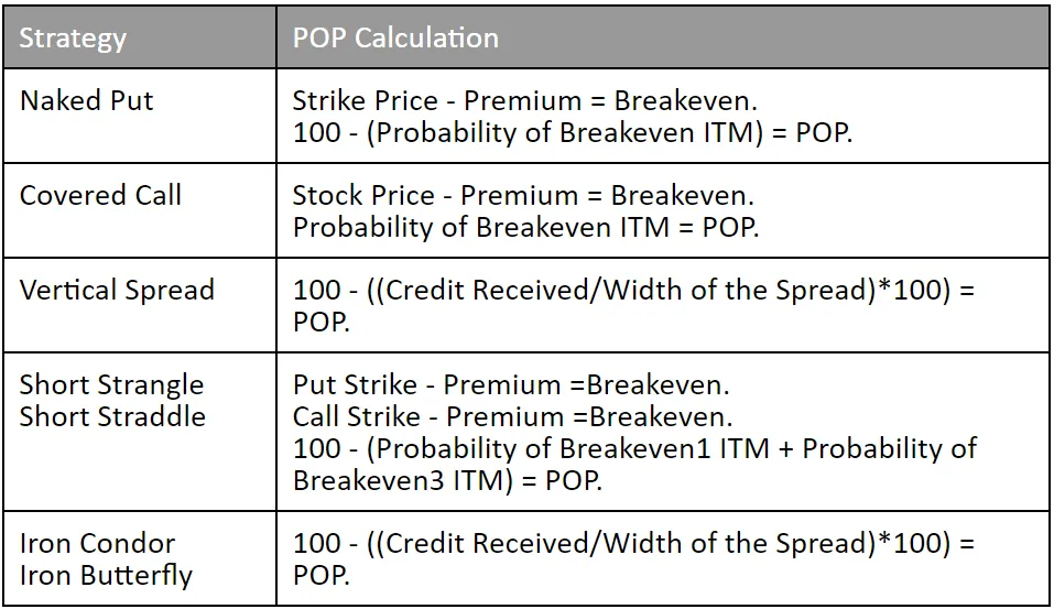
Here is a quick summary of POP calculation of few other strategies based on the above theory –
Statistically, POP can be utilized in conjunction with the statistics based strategy of having a high number of trading occurrences. At the end of the day, probabilities are probabilities. If we risk our entire account on one trade that has a POP. of 80%, we may win; however, the statistics tell us that we will lose approximately 20% of those trades over time. If one of those times happens to be now, we would be wiped out with no cash left to put on more trades!
Also, the higher the POP, the lower the profit potential. ATM options have lower POP than OTM options in terms of selling.
If two events are independent their probabilities should be multiplied, you’ve added them, how come? (think coin toss)
Hi Bard,
It depends on how you define events. In an example of tossing a coin, getting a head or tail in a single toss are two independent events. They are added together to know about their collective probability of occurence one of that events. It adds up to 1 because they are the only events, either head and tail, therefore they have to add up to 1.
But when you consider two successive tosses, and are looking for a specific events out of those two tisses, they become dependent events and their probabilities get multiplied to find out the collective probability.
Suppose we are interested in finding out the probability of getting heads in both the tosses them getting a head in the second toss is dependent on getting a head in the first toss. Therefore the collective probability becomes 0.5×0.5 = 0.25.
On the contrary if you consider another popular event of throwung a dice and interested in finding out the probability of getting an even number it will amount to adding up probability of getting either 2, 4 or 6. Here you add the three probabilities 1/6 + 1/6 + 1/6 = 3/6 = 1/2 which is as expected.