Black Scholes Model

“Black-Scholes: where risk meets reward, and math meets magic.”

The Black Scholes model is a widely used mathematical model for pricing options. It is based on the principle that the value of an option is determined by the volatility of the underlying asset, the time remaining until expiration, the strike price of the option, and the risk-free interest rate.

 In Indian share market, the Black Scholes model is used extensively for pricing options on stocks and indices.

A Brief History of Black Scholes Model

Fischer Black was born in Washington D.C. in 1938 and grew up in a family of mathematicians. His father was a mathematician and his mother was a statistician. Myron Scholes was born in Canada in 1941 and grew up in a small town called Timmins. His father was a dentist and his mother was a schoolteacher.

Both Black and Scholes earned their Ph.D.s in economics from the University of Chicago in the 1960s, where they were students of Eugene Fama, a future Nobel laureate in economics.

In the early 1970s, Black and Scholes began collaborating on a mathematical model for valuing options contracts, which became known as the Black-Scholes model. The Black-Scholes model revolutionized the field of options trading and earned Black and Scholes the Nobel Prize in Economics in 1997 (posthumously awarded to Black, who passed away in 1995).

Interestingly, while Black and Scholes are best known for their work on the Black-Scholes model, they also made significant contributions to other areas of finance, including portfolio theory and risk management.

Black was known for his unconventional thinking and willingness to challenge the status quo. He was also a voracious reader and loved science fiction and fantasy novels. Scholes, on the other hand, was known for his rigorous analytical approach and attention to detail. He was also an avid skier and sailor.

Today, the Black-Scholes model remains a cornerstone of options pricing and is widely used by traders and investors around the world.

Formulas of Black Scholes Model

The basic formula for the Black-Scholes model is:

C = SN(d1) - Ke^(-rt)N(d2)

Where:

• C is the theoretical call option price
• S is the current stock price
• K is the option’s strike price
• r is the risk-free interest rate
• t is the time until expiration
• e is the mathematical constant e (approximately equal to 2.71828)

d1 and d2 are calculated using the following formulas:

• d1 = [ln(S/K) + (r + (σ^2)/2)t] / (σ√t)
• d2 = d1 - σ√t

Where:

σ is the standard deviation of the stock’s returns

Similarly, the formula for the theoretical put option price is given by:

P = Ke^(-rt)N(-d2) - SN(-d1)

Where:

• P is the theoretical put option price
• N is the cumulative distribution function of the standard normal distribution (-∞ to x)
• -d1 and -d2 are calculated using the same formulas as for the call option price.

Black Scholes Model and Implied Volatility

1. The Black Scholes Model is based on the assumption that the volatility of the underlying asset remains constant over the life of the option. However, in reality, volatility is not constant, and this is where the concept of implied volatility comes into play. 
2. Implied volatility is the estimated volatility of an asset’s price that is implied by the market price of an option. It is a forward-looking measure that reflects the market’s expectation of the asset’s future price volatility.

And, 

1. In the Black Scholes Model, the option pricing formula is dependent on five variables: the current stock price, the exercise price of the option, the time to expiration, the risk-free interest rate, and the implied volatility. 
2. Implied volatility is the only variable that cannot be directly observed but can be estimated using the option pricing formula.

Okay, let’s break it down and revisit some important stuff we’ve already talked about to understand the relationship between Black Scholes Model and Implied Volatility in the Indian Share Market:

Factors Affecting Implied Volatility:

Implied volatility is affected by various factors, including supply and demand, market sentiment, and economic news. High demand for options typically leads to higher implied volatility, while low demand for options leads to lower implied volatility. Similarly, positive news and economic data tend to increase implied volatility, while negative news decreases implied volatility.

Implied Volatility and Trading Strategies:

Traders and investors use implied volatility to help them make trading decisions. High implied volatility can indicate a potentially attractive trading opportunity, while low implied volatility may indicate that the market is not expecting significant price movements.

Historical Volatility vs. Implied Volatility:

Historical volatility is a measure of the asset’s actual price movements in the past. It is calculated based on the asset’s past price data. Implied volatility, on the other hand, is a forward-looking estimate based on the option’s market price. Both are important in options trading, and traders use a combination of both to make informed decisions.

Calculations of Implied Volatility using Black Scholes Model

Implied volatility is an essential parameter in the Black Scholes Model, as it represents the expected volatility of the underlying asset in the future. It is also a significant factor in determining the option prices in the market. In this section, we will discuss how to calculate implied volatility using the Black Scholes Model in the Indian share market.

The implied volatility can be calculated using the following formula:

σ_imp = (2π/t)^0.5 × C/S

Where:

π is the mathematical constant π (approximately equal to 3.14159)

To derive the formula σ_imp = (2π/t)^0.5 × C/S, we start with the Black-Scholes formula for the call option price:

C = SN(d1) - Xe^(-r*t)*N(d2)

Rearranging the terms, we get:

N(d1) = (C + Xe^(-rt))/S

Taking the derivative of N(d1) with respect to σ, we get:

dN(d1)/dσ = S*sqrt(t)*exp(-d1^2/2)/sqrt(2π)

Using the chain rule, we can calculate dC/dσ as:

dC/dσ = dN(d1)/dσ * S * σ * sqrt(t)

Substituting dN(d1)/dσ, we get:

dC/dσ = S*sqrt(t)*exp(-d1^2/2)/sqrt(2π) * S * σ * sqrt(t)

Simplifying, we get:

dC/dσ = S^2texp(-d1^2/2)/sqrt(2π)

Dividing both sides by C and multiplying by σ, we get:

σ_imp = (2π/t)^0.5 × C/S

This formula shows that the implied volatility is proportional to the ratio of the option price to the stock price, and to the square root of the time to maturity. The formula can be used to calculate the implied volatility of any European call option, given the option price, the stock price, the strike price, the risk-free interest rate, and the time to maturity.

Use Implied Volatility in Black Scholes Model

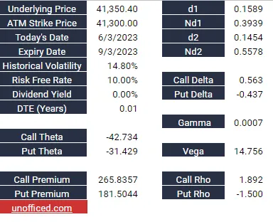
Let’s checkout an example as stated below – 

• CMP of BankNIFTY is 41350.4.
• IV of 41300PE is 14.8.
• Days to expiry is 3 days.
• Risk free Interest rate is 10%.
• Dividend is 0%.

Find the price of 41300PE. 

You can find Python code as well as detailed Spreadsheets doing the entire calculation in the Black Scholes Model. Check out here – https://unofficed.com/nse-python/black-scholes-formula-in-python/

Here is a snapshot of recent prices of 41300CE and 41300PE.

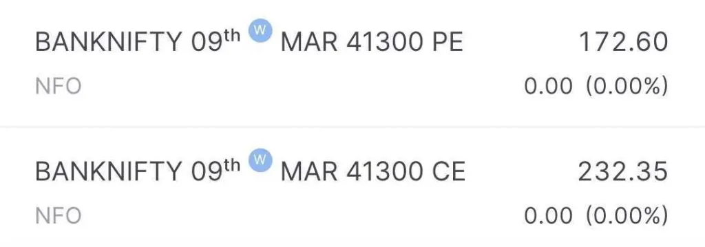
You can see the price of 41300PE is 172.6. So, We can conclude Put Options is undervalued, theoretically. 

Note, In the Black Scholes Model, 

• We can calculate the theoretical price of the option contract if the implied volatility of that option contract is given.
• Or, We can calculate the implied volatility of the option contract if the theoretical price of that option contract is given.

As per usual practice, the value of India VIX serves as the IV for all option contracts. This is because we require both to calculate the Options Greeks. While we won’t be delving too deeply into the nitty-gritty of Options Greeks calculations, feel free to check out the Python code structure and relevant discussion in the link shared above. 

So, Why not take the IV from the Options Chain of the NSE website? It is because many times, the field of IV comes blank in the website.