Backtesting Index Inside Bar Intraday Strategy Using Python

Let’s start by importing index_ib.csv file which was shared in the earlier chapter. It contains all dates when NIFTY and BankNIFTY Index exhibited Inside Bar Pattern since 2015 to today.
In case You have went through course of Coding Time Compression Scanners that shows how to scan the stocks for these bars from stratch, Please save the database to the same format and if needed add fake column entry to adjust with following tutorial –
Initialize the Database
					df = pd.read_csv("/root/apps/trident/index_ib.csv")
df
The output will be –
date	symbol	marketcapname	sector
0	01-12-2015	NIFTYFINSERVICE	Smallcap	Indices
1	01-12-2015	BANKNIFTY	Smallcap	Indices
2	07-12-2015	NIFTYFINSERVICE	Smallcap	Indices
3	10-12-2015	NIFTY	Smallcap	Indices
4	10-12-2015	NIFTYFINSERVICE	Smallcap	Indices
...	...	...	...	...
558	31-07-2023	BANKNIFTY	Smallcap	Indices
559	04-08-2023	NIFTYFINSERVICE	Smallcap	Indices
560	07-08-2023	BANKNIFTY	Smallcap	Indices
561	10-08-2023	NIFTY	Smallcap	Indices
562	17-08-2023	NIFTY	Smallcap	Indices
563 rows × 4 columns
Note that the uploaded files are sometimes updated with new files with current data. So, You may see slightly different format or more amount of data. Nothing to worry about.
Get Yesterday's High and Low and Today's Open Price
Next, we will cycle through each row of this Pandas database, applying our previously developed get_stock_data() function from the previous chapter. This function will provide us with three outputs:
- Yesterday’s high
- Yesterday’s low
- Today’s open.
We will then store these values in new columns.
					import datetime

for index, row in df.iterrows():
    symbol = row['symbol']
    time = row['date']
    high,low,today_open= get_stock_data(symbol, time)
    df.at[index, 'high'] = high
    df.at[index, 'low'] = low
    df.at[index, 'today_open'] = today_open

df
The output looks like –
					date	symbol	marketcapname	sector	high	low	today_open
0	01-12-2015	NIFTYFINSERVICE	Smallcap	Indices	0.00	0.00	0.00
1	01-12-2015	BANKNIFTY	Smallcap	Indices	17495.45	17353.85	17457.15
2	07-12-2015	NIFTYFINSERVICE	Smallcap	Indices	0.00	0.00	0.00
3	10-12-2015	NIFTY	Smallcap	Indices	7691.95	7610.00	7699.60
4	10-12-2015	NIFTYFINSERVICE	Smallcap	Indices	0.00	0.00	0.00
...	...	...	...	...	...	...	...
558	31-07-2023	BANKNIFTY	Smallcap	Indices	45694.90	45359.75	45740.00
559	04-08-2023	NIFTYFINSERVICE	Smallcap	Indices	0.00	0.00	0.00
560	07-08-2023	BANKNIFTY	Smallcap	Indices	45011.35	44773.85	44888.95
561	10-08-2023	NIFTY	Smallcap	Indices	19623.60	19495.40	19554.25
562	17-08-2023	NIFTY	Smallcap	Indices	19461.55	19326.25	19301.75
563 rows × 7 columns
Now there are some rows with `high` variable’s value as 0. Like Nifty Fin Service did not had futures data because it was not even in derivatives back then. Right? Let’s remove it.
					# Remove rows with high value of 0
df = df[df['high'] != 0]
Checking the Condition of Gap Trigger
Also Check for the Condition of Gap Triggers
In case of gap up above the previous day’s high or gap down below the previous day’s low, please avoid buying it or selling it respectively. It means –
- If there’s a gap up above the previous day’s high (the sell point), it implies that the sell trade has already been triggered, so we avoid this scenario.
- Likewise, in the case of a gap down, we steer clear of situations where there’s a gap down below the previous day’s low (the buy point).
					# Create 'gap_df' DataFrame containing rows with 'gap_trigger' as True
gap_df = df[df['gap_trigger']]

# Remove rows with 'gap_trigger' as True from the main df
df = df[df['gap_trigger'] == False]

# Reset index of both DataFrames
df.reset_index(drop=True, inplace=True)
gap_df.reset_index(drop=True, inplace=True)

print("Main DataFrame (df):")
df
The output looks –
					date	symbol	marketcapname	sector	high	low	today_open	gap_trigger
0	01-12-2015	BANKNIFTY	Smallcap	Indices	17495.45	17353.85	17457.15	False
1	31-12-2015	BANKNIFTY	Smallcap	Indices	16972.25	16896.65	16932.50	False
2	21-01-2016	NIFTY	Smallcap	Indices	7398.70	7250.00	7355.70	False
3	21-01-2016	BANKNIFTY	Smallcap	Indices	15364.60	14918.15	15343.15	False
4	15-03-2016	BANKNIFTY	Smallcap	Indices	15386.85	15268.10	15304.35	False
...	...	...	...	...	...	...	...	...
166	05-07-2023	NIFTY	Smallcap	Indices	19421.60	19339.60	19385.70	False
167	10-07-2023	NIFTY	Smallcap	Indices	19435.85	19327.10	19427.10	False
168	19-07-2023	BANKNIFTY	Smallcap	Indices	45707.40	45433.00	45689.05	False
169	07-08-2023	BANKNIFTY	Smallcap	Indices	45011.35	44773.85	44888.95	False
170	10-08-2023	NIFTY	Smallcap	Indices	19623.60	19495.40	19554.25	False
171 rows × 8 columns
gap_df database.
print(gap_df)
The output looks –
					date	symbol	marketcapname	sector	high	low	today_open	gap_trigger
0	10-12-2015	NIFTY	Smallcap	Indices	7691.95	7610.00	7699.60	True
1	23-12-2015	BANKNIFTY	Smallcap	Indices	16913.15	16812.50	16926.95	True
2	19-01-2016	NIFTY	Smallcap	Indices	7462.75	7364.15	7357.00	True
3	08-03-2016	BANKNIFTY	Smallcap	Indices	15326.65	15066.50	15022.35	True
4	29-03-2016	BANKNIFTY	Smallcap	Indices	15774.10	15580.80	15829.60	True
...	...	...	...	...	...	...	...	...
106	26-06-2023	BANKNIFTY	Smallcap	Indices	43773.10	43541.75	43804.55	True
107	05-07-2023	BANKNIFTY	Smallcap	Indices	45418.90	45073.40	45060.55	True
108	26-07-2023	BANKNIFTY	Smallcap	Indices	46096.60	45804.70	46285.85	True
109	31-07-2023	BANKNIFTY	Smallcap	Indices	45694.90	45359.75	45740.00	True
110	17-08-2023	NIFTY	Smallcap	Indices	19461.55	19326.25	19301.75	True
111 rows × 8 columns
That’s something to think about. Almost half the entries are gap triggers which is kind of considerable amount of dataset. You may explore other kind of strategies like Opening Range Breakout on those scrips.
But that is out of the purview of the current discussion. Anyways, let’s remove the gap_trigger, marketcapname, and sector columns because they are not needed.
					# Remove columns 'gap_trigger', 'marketcapname', and 'sector'
df.drop(['gap_trigger', 'marketcapname', 'sector'], axis=1, inplace=True)
That’s something to think about. Almost half the entries are gap triggers which is kind of considerable amount of dataset. You may explore other kind of strategies like Opening Range Breakout on those scrips.
But that is out of the purview of the current discussion. Anyways, let’s remove the gap_trigger, marketcapname, and sector columns because they are not needed.
Setting the Target
This strategy already incorporates a built-in trigger and stop-loss mechanism. Here’s a concise explanation which we have already discussed earlier:
The stock’s high price plays a dual role:
- It acts as the stop-loss level when executing a sell trade.
- It serves as the trigger point to initiate a buy trade.
Similarly, the low price of the stock has its significance:
- It functions as the stop-loss level for buy trades once the buy order is placed.
- It serves as the trigger point for entering a sell trade.
In summary:
- High of the stock = Buy Trigger = Sell Stoploss
- Low of the stock = Sell Trigger = Buy Stoploss
Since this strategy inherently determines entry and stop-loss levels from the candlesticks, let’s now focus on defining profit targets. We’ll set the risk-reward ratio at 1:3 as a starting point.
Feel free to experiment with different risk-reward ratios, such as 1:5 or others, to further explore the strategy’s dynamics.
					# Calculate and add buy_target and sell_target columns
df['buy_target'] = df['today_open'] + 3 * (df['high'] - df['low'])
df['sell_target'] = df['today_open'] - 3 * (df['high'] - df['low'])
df
The output looks like –
					date	symbol	high	low	today_open	buy_target	sell_target
0	01-12-2015	BANKNIFTY	17495.45	17353.85	17457.15	17881.95	17032.35
1	31-12-2015	BANKNIFTY	16972.25	16896.65	16932.50	17159.30	16705.70
2	21-01-2016	NIFTY	7398.70	7250.00	7355.70	7801.80	6909.60
3	21-01-2016	BANKNIFTY	15364.60	14918.15	15343.15	16682.50	14003.80
4	15-03-2016	BANKNIFTY	15386.85	15268.10	15304.35	15660.60	14948.10
...	...	...	...	...	...	...	...
166	05-07-2023	NIFTY	19421.60	19339.60	19385.70	19631.70	19139.70
167	10-07-2023	NIFTY	19435.85	19327.10	19427.10	19753.35	19100.85
168	19-07-2023	BANKNIFTY	45707.40	45433.00	45689.05	46512.25	44865.85
169	07-08-2023	BANKNIFTY	45011.35	44773.85	44888.95	45601.45	44176.45
170	10-08-2023	NIFTY	19623.60	19495.40	19554.25	19938.85	19169.65
171 rows × 7 columns
Run The Buddha Backtester Function
Now that We have the following variables,
symbol: The stock symbol (e.g., “RELIANCE”).time: A time parameter (currently unused within the function).high: The stock’s high price.low: The stock’s low price.buy_target: The buy target price.sell_target: The sell target price.
Let’s run the check_high_breakout_and_save function we designed in our earlier chapter. This Python function is designed to scan historical stock price data and assess whether buy and sell trades are triggered, monitor trade targets and stop losses, calculate profits and losses, and manage trade exits.
					import datetime
from pprint import pprint

# Iterate through the DataFrame and update 'entry_time' column
for index, row in df.iterrows():
    symbol = row['symbol']
    time = row['date']
    high = row['high']
    low = row['low']
    buy_target = row['buy_target']
    sell_target = row['sell_target']

    buy_trigger,sell_trigger,buy_trigger_stoploss,sell_trigger_stoploss,buy_exit_time,buy_exit_price,sell_exit_time,sell_exit_price,buy_trigger_target,sell_trigger_target,buy_pl_points,sell_pl_points = check_high_breakout_and_save(symbol, time,high,low,buy_target,sell_target)
    df.at[index, 'buy_trigger'] = buy_trigger
    df.at[index, 'sell_trigger'] = sell_trigger
    df.at[index, 'buy_trigger_stoploss'] = buy_trigger_stoploss
    df.at[index, 'sell_trigger_stoploss'] = sell_trigger_stoploss
    df.at[index, 'buy_exit_time'] = buy_exit_time
    df.at[index, 'buy_exit_price'] = buy_exit_price
    df.at[index, 'sell_exit_time'] = sell_exit_time
    df.at[index, 'sell_exit_price'] = sell_exit_price
    df.at[index, 'buy_trigger_target'] = buy_trigger_target
    df.at[index, 'sell_trigger_target'] = sell_trigger_target
    df.at[index, 'buy_pl_points'] = buy_pl_points
    df.at[index, 'sell_pl_points'] = sell_pl_points


df
The output looks like –
						date	symbol	high	low	today_open	buy_target	sell_target	buy_trigger	sell_trigger	buy_trigger_stoploss	sell_trigger_stoploss	buy_exit_time	buy_exit_price	sell_exit_time	sell_exit_price	buy_trigger_target	sell_trigger_target	buy_pl_points	sell_pl_points
0	01-12-2015	BANKNIFTY	17495.45	17353.85	17457.15	17881.95	17032.35	0.0	2015-12-02 09:54:00	0.0	0.0	0.0	0.00	2015-12-02 14:20:00	17185.45	0.0	0.0	0.00	168.40
1	31-12-2015	BANKNIFTY	16972.25	16896.65	16932.50	17159.30	16705.70	2016-01-01 13:41:00	2016-01-01 09:21:00	0.0	2016-01-01 13:41:00	2016-01-01 14:20:00	17046.40	0	0.00	0.0	0.0	74.15	-75.60
2	21-01-2016	NIFTY	7398.70	7250.00	7355.70	7801.80	6909.60	2016-01-22 11:00:00	0	0.0	0	2016-01-22 14:20:00	7421.35	0	0.00	0.0	0.0	22.65	0.00
3	21-01-2016	BANKNIFTY	15364.60	14918.15	15343.15	16682.50	14003.80	2016-01-22 10:01:00	0	0.0	0	2016-01-22 14:20:00	15533.05	0	0.00	0.0	0.0	168.45	0.00
4	15-03-2016	BANKNIFTY	15386.85	15268.10	15304.35	15660.60	14948.10	0	2016-03-16 10:40:00	0.0	0	0	0.00	2016-03-16 14:20:00	15276.65	0.0	0.0	0.00	-8.55
...	...	...	...	...	...	...	...	...	...	...	...	...	...	...	...	...	...	...	...
166	05-07-2023	NIFTY	19421.60	19339.60	19385.70	19631.70	19139.70	2023-07-06 09:30:00	0	0	0	2023-07-06 14:20:00	19484.50	0	0.00	0	0.0	62.90	0.00
167	10-07-2023	NIFTY	19435.85	19327.10	19427.10	19753.35	19100.85	2023-07-11 09:20:00	0	0	0	2023-07-11 14:20:00	19446.25	0	0.00	0	0.0	10.40	0.00
168	19-07-2023	BANKNIFTY	45707.40	45433.00	45689.05	46512.25	44865.85	2023-07-20 09:23:00	0	0	0	2023-07-20 14:20:00	46126.35	0	0.00	0	0.0	418.95	0.00
169	07-08-2023	BANKNIFTY	45011.35	44773.85	44888.95	45601.45	44176.45	2023-08-08 10:25:00	0	0	0	2023-08-08 14:20:00	44953.35	0	0.00	0	0.0	-58.00	0.00
170	10-08-2023	NIFTY	19623.60	19495.40	19554.25	19938.85	19169.65	0	2023-08-11 09:20:00	0	0	0	0.00	2023-08-11 14:20:00	19471.05	0	0.0	0.00	24.35
171 rows × 19 columns
The backtest is complete. Now, it is time to visualize the data in an easier way. With graphs along with various analytics.
Run Various Performance Metrics
					import pandas as pd

# Assuming df is your DataFrame

# Calculate net of buy_pl_points and sell_pl_points
net_buy_pl = df['buy_pl_points'].sum()
net_sell_pl = df['sell_pl_points'].sum()

# Calculate positive, negative, and total occurrences of buy_pl_points
positive_buy_count = (df['buy_pl_points'] > 0).sum()
negative_buy_count = (df['buy_pl_points'] < 0).sum()
total_buy_count = df['buy_pl_points'].count()

# Calculate positive, negative, and total occurrences of sell_pl_points
positive_sell_count = (df['sell_pl_points'] > 0).sum()
negative_sell_count = (df['sell_pl_points'] < 0).sum()
total_sell_count = df['sell_pl_points'].count()

# Print the calculated metrics
print("Net of buy_pl_points:", net_buy_pl)
print("Net of sell_pl_points:", net_sell_pl)
print("Positive buy_pl_points count:", positive_buy_count)
print("Negative buy_pl_points count:", negative_buy_count)
print("Total buy_pl_points count:", total_buy_count)
print("Positive sell_pl_points count:", positive_sell_count)
print("Negative sell_pl_points count:", negative_sell_count)
print("Total sell_pl_points count:", total_sell_count)
This code snippet calculates and analyzes various trading performance metrics from a given DataFrame.
- Net Profit and Loss Calculation: It calculates the net profit (
net_buy_pl) and net loss (net_sell_pl) by summing up all the buy and sell profit/loss points, respectively. - Buy Profit Points Analysis: It computes the count of positive buy profit points (profits) as
positive_buy_count, the count of negative buy profit points (losses) asnegative_buy_count, and the total count of buy profit points astotal_buy_count. - Sell Profit Points Analysis: Similar to the buy analysis, it calculates the count of positive sell profit points (profits) as
positive_sell_count, the count of negative sell profit points (losses) asnegative_sell_count, and the total count of sell profit points astotal_sell_count.
					Net of buy_pl_points: 2221.00000000001
Net of sell_pl_points: 4721.430000000011
Positive buy_pl_points count: 46
Negative buy_pl_points count: 27
Total buy_pl_points count: 171
Positive sell_pl_points count: 60
Negative sell_pl_points count: 24
Total sell_pl_points count: 171
Adding the Lot Size
Since the code currently calculates profits in points, it’s essential to incorporate lot size information to determine the quantity. Without specifying the quantity, it becomes challenging to interpret the profit amount and other associated metrics.
However, it’s worth noting that lot sizes can vary over time due to SEBI’s discretion. To address this, we’ll temporarily fix the current lot size within the system and compute profits across the entire dataset while normalizing it. While this approach may be considered unethical for backtesting purposes, the small sample size shouts that the resulting deviation in the output will be negligible and inconsequential.
					def calculate_lotsize(row):
    if row["symbol"] == "BANKNIFTY":
        return 15
    elif row["symbol"] == "NIFTY":
        return 50
    else:
        return 40

df["lotsize"] = df.apply(calculate_lotsize, axis=1)
df["buy_pl_points"] = df["buy_pl_points"]*df["lotsize"]
df["sell_pl_points"] = df["sell_pl_points"]*df["lotsize"]
Running More Performance Metrics
Since We have the quantity in place. Let’s get these following metrics –
- Average of all buy_pl_points: This is the average profit or loss for all buy trades.
- Average of all sell_pl_points: This is the average profit or loss for all sell trades.
- Average of positive buy_pl_points: This is the average profit for buy trades that resulted in a profit.
- Average of positive sell_pl_points: This is the average profit for sell trades that resulted in a profit.
- Average of negative buy_pl_points: This is the average loss for buy trades that resulted in a loss.
- Average of negative sell_pl_points: This is the average loss for sell trades that resulted in a loss.
# Assuming df is your DataFrame

# Calculate average of buy_pl_points and sell_pl_points
average_buy_pl = df['buy_pl_points'].mean()
average_sell_pl = df['sell_pl_points'].mean()

# Calculate average of positive buy_pl_points and positive sell_pl_points
average_positive_buy_pl = df.loc[df['buy_pl_points'] > 0, 'buy_pl_points'].mean()
average_positive_sell_pl = df.loc[df['sell_pl_points'] > 0, 'sell_pl_points'].mean()

# Calculate average of negative buy_pl_points and negative sell_pl_points
average_negative_buy_pl = df.loc[df['buy_pl_points'] < 0, 'buy_pl_points'].mean()
average_negative_sell_pl = df.loc[df['sell_pl_points'] < 0, 'sell_pl_points'].mean()

# Print the calculated averages
print("Average of buy_pl_points:", average_buy_pl)
print("Average of sell_pl_points:", average_sell_pl)
print("Average of positive buy_pl_points:", average_positive_buy_pl)
print("Average of positive sell_pl_points:", average_positive_sell_pl)
print("Average of negative buy_pl_points:", average_negative_buy_pl)
print("Average of negative sell_pl_points:", average_negative_sell_pl)
					Average of buy_pl_points: 347.5760233918145
Average of sell_pl_points: 563.6125730994178
Average of positive buy_pl_points: 2607.565217391311
Average of positive sell_pl_points: 2375.0291666666717
Average of negative buy_pl_points: -2241.203703703704
Average of negative sell_pl_points: -1921.8333333333273
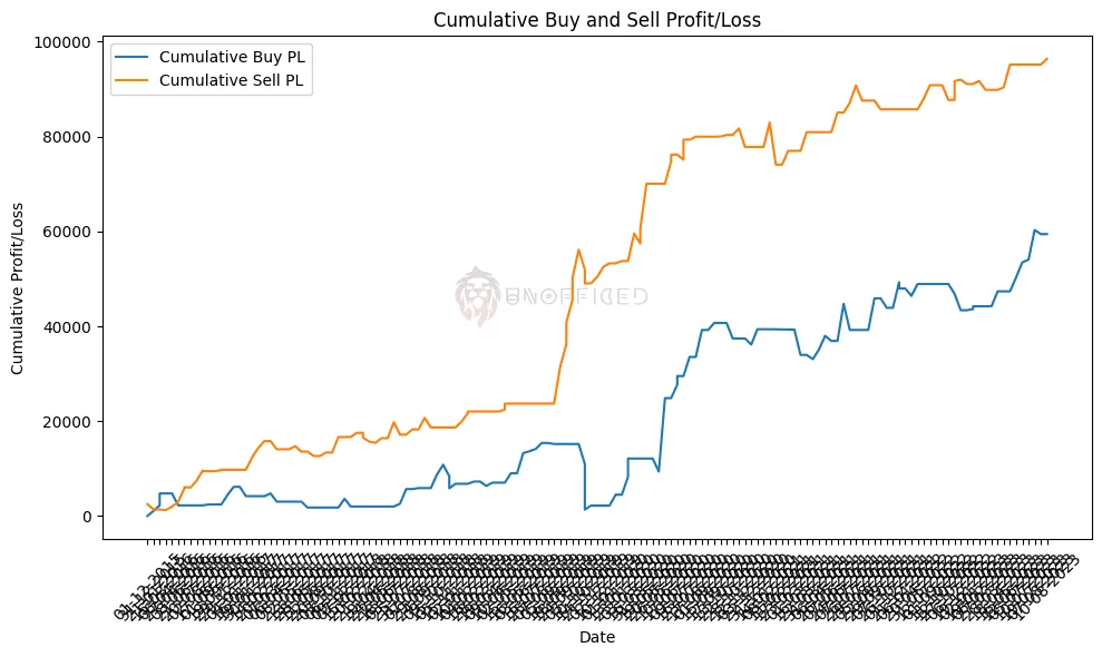
Plotting the Equity Curve
The following code calculates the cumulative profit and loss (PL) over time for both buy and sell trades using the ‘buy_pl_points‘ and ‘sell_pl_points‘ columns in a DataFrame. It creates a line plot that represents the equity curve, also known as the cumulative PL versus time.
In this plot, the x-axis represents time (in this case, dates), and the y-axis represents the cumulative profit or loss. The ‘Cumulative Buy PL‘ line shows the cumulative profit or loss for all buy trades over the given time period, while the ‘Cumulative Sell PL‘ line shows the cumulative profit or loss for all sell trades over the same period.
					import pandas as pd
import matplotlib.pyplot as plt

# Assuming df is your DataFrame

# Calculate cumulative sum of buy_pl_points and sell_pl_points
df['cumulative_buy_pl'] = df['buy_pl_points'].cumsum()
df['cumulative_sell_pl'] = df['sell_pl_points'].cumsum()

# Create a line plot
plt.figure(figsize=(10, 6))
plt.plot(df['date'], df['cumulative_buy_pl'], label='Cumulative Buy PL')
plt.plot(df['date'], df['cumulative_sell_pl'], label='Cumulative Sell PL')
plt.xlabel('Date')
plt.ylabel('Cumulative Profit/Loss')
plt.title('Cumulative Buy and Sell Profit/Loss')
plt.legend()
plt.xticks(rotation=45)
plt.tight_layout()
plt.show()
This equity curve provides a visual representation of how the trading strategy has performed over time, allowing you to see trends, fluctuations, and the overall profitability of the strategy.
It helps traders and analysts assess the strategy’s performance and make informed decisions based on historical data.