Transforming Candlesticks OHLC into Heikin-Ashi Using Python

This is a programming lesson. So there will be very less amount of explanation and more code. If you’re stuck somewhere, feel free to comment.
Objective
Converting a dataframe that has Open, High, Low, Close of Candlestick data to Heiken Ashi
Note – The structure of historical data and live data from Zerodha is identical. During the development and testing of functions, it’s not feasible to wait for days or months to validate their performance using live data.
To address this, we’ll initially test and validate our functions using historical data. Once we have confirmed that the functions generate accurate signals and execute trades correctly with historical data, we can seamlessly transition to using live data for real-time trading.
Objective
The Heikin-Ashi technique, deriving its name from the Japanese term for “average bar,” is a unique method used alongside traditional candlestick charts in financial markets. This technique plays a crucial role in identifying market trends and forecasting future prices, making it invaluable for traders aiming to capitalize on market movements.
Understanding Heikin-Ashi
Heikin-Ashi charts differ from standard candlestick charts, although they retain some similarities. The primary distinction lies in the calculation method, which smooths out price data, thereby facilitating trend identification and analysis. This smoothing effect can help traders remain in trades during sustained trends and alert them to exit when trends show signs of reversal.
Key Takeaways:
Trend Identification and Analysis: The primary application of Heikin-Ashi is to assist traders in spotting and analyzing market trends. This technique simplifies the process of reading candlestick charts, making trends more discernible.
Primary Signals: There are five main signals in Heikin-Ashi charts that traders rely on to interpret market movements. These signals provide insights into market trends and potential reversals.
Versatility: Heikin-Ashi charts are adaptable and can be employed in various markets, underlining their versatility in different trading environments.
The Heikin-Ashi Formula:
The Heikin-Ashi technique modifies the traditional open-high-low-close (OHLC) values used in candlestick charts, creating a unique formula:
Normal candlestick charts are composed of a series of open-high-low-close (OHLC) candles set apart by a time series. The Heikin-Ashi technique shares some characteristics with standard candlestick charts but uses a modified formula of close-open-high-low (COHL):
\( \text{Close} = \frac{1}{4} (\text{Open} + \text{High} + \text{Low} + \text{Close}) \)
This is calculated as the average of the open, high, low, and close prices of the current bar.
\( \text{Open} = \frac{1}{2} (\text{Open of Prev. Bar} + \text{Close of Prev. Bar}) \)
The opening price of a Heikin-Ashi bar is the midpoint of the previous bar.
\( \text{High} = \text{Max}[\text{High}, \text{Open}, \text{Close}] \)
The high of a Heikin-Ashi bar is the maximum value among the current high, open, and close.
\( \text{Low} = \text{Min}[\text{Low}, \text{Open}, \text{Close}] \)
Conversely, the low is the minimum value among the current low, open, and close.
					import datetime
starting_date=datetime.datetime(2019, 1, 1)
ending_date=datetime.datetime.today()

token = "738561" #Reliance Token

zap=kite.historical_data(token,starting_date,ending_date,"day")
zap= pd.DataFrame(zap)
print(zap.head(10))
Output –
					   date     open     high      low    close   volume
0 2019-01-01 00:00:00+05:30  1072.60  1074.55  1058.15  1068.55  4674623
1 2019-01-02 00:00:00+05:30  1062.35  1074.25  1049.45  1054.60  7495774
2 2019-01-03 00:00:00+05:30  1055.65  1062.45  1039.05  1041.60  7812063
3 2019-01-04 00:00:00+05:30  1046.05  1052.75  1030.50  1047.25  8880762
4 2019-01-07 00:00:00+05:30  1055.20  1066.10  1049.45  1053.05  5784264
5 2019-01-08 00:00:00+05:30  1053.35  1058.00  1044.70  1052.95  5901337
6 2019-01-09 00:00:00+05:30  1059.95  1064.70  1047.30  1058.75  6049944
7 2019-01-10 00:00:00+05:30  1055.90  1059.00  1051.40  1055.65  4280617
8 2019-01-11 00:00:00+05:30  1055.75  1061.65  1037.65  1046.65  6781268
9 2019-01-14 00:00:00+05:30  1043.75  1049.00  1035.55  1045.45  4313662
Now that we got ‘zap’ which is your DataFrame with OHLC data. Even with live data stream, You can convert that to this dataframe easily.
					def calculate_heikin_ashi(data):
    ha_close = (data['open'] + data['high'] + data['low'] + data['close']) / 4
    ha_open = (data['open'].shift(1) + data['close'].shift(1)) / 2
    ha_high = data[['high', 'close', 'open']].max(axis=1)
    ha_low = data[['low', 'close', 'open']].min(axis=1)

    ha_data = pd.DataFrame({'Date': data['date'], 'Open': ha_open, 'Close': ha_close, 'High': ha_high, 'Low': ha_low, 'Volume': data['volume']})

    return ha_data

zap_ashi = calculate_heikin_ashi(zap)

print(zap_ashi.head(10))
The initial open value for the first Heiken Ashi candlestick cannot be determined using the standard Heiken Ashi formula, as this calculation requires data from the previous day, which is not available for the first candlestick in a series.
It is showing as nan as you can see here.
Output –
					            Date      Open      Close     High      Low   Volume
0 2019-01-01 00:00:00+05:30       NaN  1068.4625  1074.55  1058.15  4674623
1 2019-01-02 00:00:00+05:30  1070.575  1060.1625  1074.25  1049.45  7495774
2 2019-01-03 00:00:00+05:30  1058.475  1049.6875  1062.45  1039.05  7812063
3 2019-01-04 00:00:00+05:30  1048.625  1044.1375  1052.75  1030.50  8880762
4 2019-01-07 00:00:00+05:30  1046.650  1055.9500  1066.10  1049.45  5784264
5 2019-01-08 00:00:00+05:30  1054.125  1052.2500  1058.00  1044.70  5901337
6 2019-01-09 00:00:00+05:30  1053.150  1057.6750  1064.70  1047.30  6049944
7 2019-01-10 00:00:00+05:30  1059.350  1055.4875  1059.00  1051.40  4280617
8 2019-01-11 00:00:00+05:30  1055.775  1050.4250  1061.65  1037.65  6781268
9 2019-01-14 00:00:00+05:30  1051.200  1043.4375  1049.00  1035.55  4313662
Plot Heiken Ashi Candlestick Graph
Now, before plotting we need to remove the rows with NaN values.
					import pandas as pd
import mplfinance as mpf

# Remove rows with NaN values
zap_ashi.dropna(inplace=True)

# Assuming 'zap_ashi' is your DataFrame
# Convert the 'date' column to datetime and set it as index
zap_ashi['Date'] = pd.to_datetime(zap_ashi['Date'])
zap_ashi.set_index('Date', inplace=True)

# Plotting the candlestick chart
mpf.plot(zap_ashi, type='candle', style='charles', title="Candlestick Chart", volume=True)
Output –
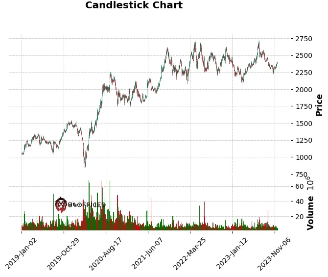
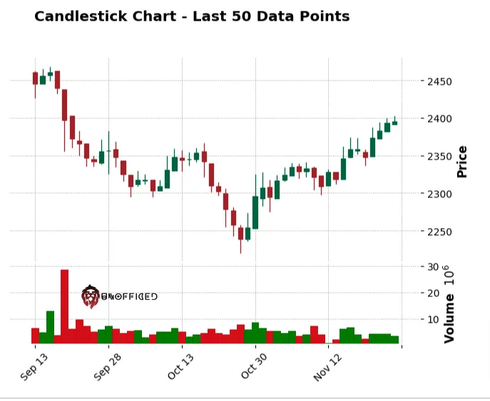
It is plotting to much data. can it plot last 50 datapoints so that we can visualize the output properly?
					import pandas as pd
import mplfinance as mpf

# Assuming 'zap_ashi' is your DataFrame
# Convert the 'date' column to datetime and set it as index
zap_ashi['Date'] = pd.to_datetime(zap_ashi['Date'])
zap_ashi.set_index('Date', inplace=True)

# Slicing the DataFrame to get the last 50 rows
last_50_rows = zap_ashi.tail(50)

# Plotting the candlestick chart for the last 50 data points
mpf.plot(last_50_rows, type='candle', style='charles', title="Candlestick Chart - Last 50 Data Points", volume=True)
Output –