Exploring Technical Indicators in the Indian Stock Market with Zerodha API and Python

This is a programming lesson. So there will be very less amount of explanation and more code. If you’re stuck somewhere, feel free to comment.
What Is a Technical Indicator?
Technical indicators are heuristic or mathematical calculations that rely on a security’s price, volume, or open interest, often employed by traders who adhere to technical analysis principles.
These indicators serve as tools for predicting future price movements by scrutinizing historical data. Some widely used technical indicators encompass the Relative Strength Index, Money Flow Index, Stochastics, MACD, and Bollinger Bands®.
How Technical Indicators Works?
Technical analysis is a trading discipline that involves the evaluation of investments and the identification of trading opportunities by analyzing statistical trends derived from trading activities, such as price movements and trading volumes. In contrast to fundamental analysts, who assess a security’s intrinsic value based on financial and economic data, technical analysts concentrate on patterns in price movements, trading signals, and a variety of analytical charting tools to gauge a security’s strength or weakness.
This approach to analysis can be applied to any security with historical trading data, encompassing stocks, futures, commodities, fixed-income instruments, currencies, and other financial assets. While we primarily focus on stocks in our examples in this tutorial, it’s essential to recognize that these concepts are universally applicable. In fact, technical analysis finds more extensive use in commodities and forex markets, where traders are primarily concerned with short-term price fluctuations.
Technical indicators, often referred to as “technicals,” center their analysis on historical trading data, including price, volume, and open interest, rather than delving into a company’s fundamentals like earnings, revenue, or profit margins. These indicators are particularly popular among active traders because they are tailored to analyze short-term price movements. However, even long-term investors can utilize technical indicators to pinpoint optimal entry and exit points.
There are two fundamental categories of technical indicators:
Overlays: These technical indicators use the same scale as prices and are plotted directly over the price chart. Notable examples include moving averages and Bollinger Bands®.
Oscillators: Oscillators are technical indicators that fluctuate between a local minimum and maximum and are typically plotted either above or below a price chart. Prominent examples encompass the stochastic oscillator, MACD (Moving Average Convergence Divergence), and RSI (Relative Strength Index).
Note – The structure of historical data and live data from Zerodha is identical. During the development and testing of functions, it’s not feasible to wait for days or months to validate their performance using live data.
To address this, we’ll initially test and validate our functions using historical data. Once we have confirmed that the functions generate accurate signals and execute trades correctly with historical data, we can seamlessly transition to using live data for real-time trading.
Python Code
					'''
    # Date must be present as a Pandas DataFrame with ['date', 'open', 'high', 'low', 'close', 'volume'] as columns
    df = pd.DataFrame(data["data"]["candles"], columns=['date', 'open', 'high', 'low', 'close', 'volume'])
'''
df=pd.DataFrame(kite.historical_data(779521,"2019-04-14 15:00:00","2019-08-16 09:16:00","day",0))[["date","open","high","low","close","volume"]]
display(df.tail(10))
Output –
					date	open	high	low	close	volume
73	2019-08-01 00:00:00+05:30	330.80	331.50	311.35	317.15	40853304
74	2019-08-02 00:00:00+05:30	315.55	322.25	307.05	308.45	64472348
75	2019-08-05 00:00:00+05:30	298.45	302.85	291.70	300.25	48815899
76	2019-08-06 00:00:00+05:30	298.80	304.25	297.25	301.40	30442970
77	2019-08-07 00:00:00+05:30	302.40	302.45	288.80	289.90	30820114
78	2019-08-08 00:00:00+05:30	290.00	295.50	285.60	294.35	32929233
79	2019-08-09 00:00:00+05:30	296.30	298.00	290.05	291.35	23377581
80	2019-08-13 00:00:00+05:30	290.90	291.55	282.50	283.35	24231272
81	2019-08-14 00:00:00+05:30	285.05	291.25	284.50	289.75	18523649
82	2019-08-16 00:00:00+05:30	287.95	292.80	284.30	290.90	20047399
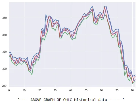
Ploting data
					plt.style.use('seaborn')
df['high'].plot()
df['low'].plot()
df['close'].plot()
df['open'].plot()
plt.show()
print ("  \t'---- ABOVE GRAPH OF OHLC Historical data ----- ' \n \n ")
Output –
Indicators
ATR (Average True Range)
- ATR measures market volatility, aiding in setting stop-loss levels.
- It quantifies potential price swings by considering the true range of price movements.
- Traders use ATR to adjust risk management strategies in varying market conditions.
					"""
Function to compute Average True Range (ATR)

Args :
    df : Pandas DataFrame which contains ['date', 'open', 'high', 'low', 'close', 'volume'] columns
    period : Integer indicates the period of computation in terms of number of candles
    ohlc: List defining OHLC Column names (default ['Open', 'High', 'Low', 'Close'])

Returns :
    df : Pandas DataFrame with new columns added for
        True Range (TR)
        ATR (ATR_$period)
"""

def atr(df,period):
    df['hl']=abs(df['high']-df['low'])
    df['hpc']=abs(df['high']-df['close'].shift())
    df['lpc']=abs(df['low']-df['close'].shift())
    df['tr']=df[['hl','hpc','lpc']].max(axis=1)
    df['ATR']=pd.DataFrame.ewm(df["tr"], span=period,min_periods=period).mean()
    df.drop(["hl","hpc","lpc","tr"],axis = 1 , inplace =True)
atr(df,14)
df.tail()
Output –
					date	open	high	low	close	volume	ATR
78	2019-08-08 00:00:00+05:30	290.00	295.50	285.60	294.35	32929233	11.851230
79	2019-08-09 00:00:00+05:30	296.30	298.00	290.05	291.35	23377581	11.331060
80	2019-08-13 00:00:00+05:30	290.90	291.55	282.50	283.35	24231272	11.026916
81	2019-08-14 00:00:00+05:30	285.05	291.25	284.50	289.75	18523649	10.609991
82	2019-08-16 00:00:00+05:30	287.95	292.80	284.30	290.90	20047399	10.328657
RSI (Relative Strength Index)
- RSI assesses the momentum of an asset on a scale of 0 to 100.
- Values above 70 indicate overbought conditions, while values below 30 suggest oversold conditions.
- It’s a popular tool for identifying potential trend reversals and entry/exit points.
					"""
    Function to compute Relative Strength Index (RSI)

    Args :
        df : Pandas DataFrame which contains ['date', 'open', 'high', 'low', 'close', 'volume'] columns
        period : Integer indicates the period of computation in terms of number of candles

    Returns :
        df : Pandas DataFrame with new columns added for
            Relative Strength Index (RSI_$period)
    """

rsi_period=14
chg=df["close"].diff(1)
gain=chg.mask(chg<0,0)
loss=chg.mask(chg>0,0)
avg_gain=gain.ewm(com=rsi_period-1,min_periods=rsi_period).mean()
avg_loss=loss.ewm(com=rsi_period-1,min_periods=rsi_period).mean()
rs =abs(avg_gain / avg_loss)
rsi =100 -(100/(1+rs))
df['rsi']=rsi
display(df.tail())
Output –
date	open	high	low	close	volume	ATR	rsi
78	2019-08-08 00:00:00+05:30	290.00	295.50	285.60	294.35	32929233	11.851230	26.529639
79	2019-08-09 00:00:00+05:30	296.30	298.00	290.05	291.35	23377581	11.331060	25.567214
80	2019-08-13 00:00:00+05:30	290.90	291.55	282.50	283.35	24231272	11.026916	23.154909
81	2019-08-14 00:00:00+05:30	285.05	291.25	284.50	289.75	18523649	10.609991	28.931857
82	2019-08-16 00:00:00+05:30	287.95	292.80	284.30	290.90	20047399	10.328657	29.950888
SMA (simple moving average)
- SMA calculates the average price over a specified time period.
- It helps smooth price data, making trends more apparent.
- Traders use SMAs to identify trend direction and potential support/resistance levels.
					"""
    Function to compute Simple Moving Average (SMA)

    Args :
        df : Pandas DataFrame which contains ['date', 'open', 'high', 'low', 'close', 'volume'] columns
        base : String indicating the column name from which the SMA needs to be computed from
        target : String indicates the column name to which the computed data needs to be stored
        period : Integer indicates the period of computation in terms of number of candles

    Returns :
        df : Pandas DataFrame with new column added with name 'target'
    """

def SMA(df, column="close", period=14):
    smavg = df.close.rolling(14).mean()
    return df.join(smavg.to_frame('SMA'))
a=SMA(df)
a.tail()
Output –
date	open	high	low	close	volume	ATR	rsi	SMA
78	2019-08-08 00:00:00+05:30	290.00	295.50	285.60	294.35	32929233	11.851230	26.529639	323.685714
79	2019-08-09 00:00:00+05:30	296.30	298.00	290.05	291.35	23377581	11.331060	25.567214	319.435714
80	2019-08-13 00:00:00+05:30	290.90	291.55	282.50	283.35	24231272	11.026916	23.154909	315.232143
81	2019-08-14 00:00:00+05:30	285.05	291.25	284.50	289.75	18523649	10.609991	28.931857	311.671429
82	2019-08-16 00:00:00+05:30	287.95	292.80	284.30	290.90	20047399	10.328657	29.950888	308.071429
EMA (Exponential Moving Average)
- EMA gives more weight to recent prices, reacting faster to market changes.
- It’s favored by traders for quicker trend identification.
- EMA crossovers are often used to signal potential entry or exit points.
					"""
    Function to compute Exponential Moving Average (EMA)
    Args :
        df : Pandas DataFrame which contains ['date', 'open', 'high', 'low', 'close', 'volume'] columns
        base : String indicating the column name from which the EMA needs to be computed from
        target : String indicates the column name to which the computed data needs to be stored
        period : Integer indicates the period of computation in terms of number of candles
        alpha : Boolean if True indicates to use the formula for computing EMA using alpha (default is False)
    Returns :
        df : Pandas DataFrame with new column added with name 'target'
    """
def EMA(df, column="close", period=14):
    ema = df[column].ewm(span=period, min_periods=period - 1).mean()
    return df.join(ema.to_frame('EMA'))
pp= ( EMA(df)["EMA"].shift(1)*13 + df['close'] ) /  14
pp.tail()
Output –
					78    321.111774
79    317.329208
80    313.293848
81    309.758441
82    307.172770
dtype: float64
Bollinger band
- Bollinger Bands® consist of three lines: a middle SMA and upper/lower bands.
- They expand and contract with price volatility, providing insights into potential price reversals.
- Traders use them to gauge volatility and identify potential breakout points.
					def BollingerBand(df, column="close", period=20):
    sma = df[column].rolling(window=period, min_periods=period - 1).mean()
    std = df[column].rolling(window=period, min_periods=period - 1).std()
    up = (sma + (std * 2)).to_frame('BBANDUP')
    lower = (sma - (std * 2)).to_frame('BBANDLO')
    return df.join(up).join(lower)
c=BollingerBand(df)
c.tail()
Output –
						date	open	high	low	close	volume	ATR	rsi	BBANDUP	BBANDLO
78	2019-08-08 00:00:00+05:30	290.00	295.50	285.60	294.35	32929233	11.851230	26.529639	387.024069	284.140931
79	2019-08-09 00:00:00+05:30	296.30	298.00	290.05	291.35	23377581	11.331060	25.567214	385.242185	278.697815
80	2019-08-13 00:00:00+05:30	290.90	291.55	282.50	283.35	24231272	11.026916	23.154909	383.881457	272.388543
81	2019-08-14 00:00:00+05:30	285.05	291.25	284.50	289.75	18523649	10.609991	28.931857	379.931275	268.878725
82	2019-08-16 00:00:00+05:30	287.95	292.80	284.30	290.90	20047399	10.328657	29.950888	372.909758	267.750242
Heiken Ashi
- Heiken Ashi charts smooth out price fluctuations, helping traders visualize trends.
- Candlestick patterns on Heiken Ashi charts differ from traditional candlesticks.
- They are useful for filtering noise in price data and identifying trend changes.
def HA(df, ohlc=['Open', 'High', 'Low', 'Close']):
    """
    Function to compute Heiken Ashi Candles (HA)
    Args :
        df : Pandas DataFrame which contains ['date', 'open', 'high', 'low', 'close', 'volume'] columns
        ohlc: List defining OHLC Column names (default ['Open', 'High', 'Low', 'Close'])
    Returns :
        df : Pandas DataFrame with new columns added for
            Heiken Ashi Close (HA_$ohlc[3])
            Heiken Ashi Open (HA_$ohlc[0])
            Heiken Ashi High (HA_$ohlc[1])
            Heiken Ashi Low (HA_$ohlc[2])
    """
    ha_open = 'HA_' + ohlc[0]
    ha_high = 'HA_' + ohlc[1]
    ha_low = 'HA_' + ohlc[2]
    ha_close = 'HA_' + ohlc[3]
    df[ha_close] = (df[ohlc[0]] + df[ohlc[1]] + df[ohlc[2]] + df[ohlc[3]]) / 4
    df[ha_open] = 0.00
    for i in range(0, len(df)):
        if i == 0:
            df[ha_open].iat[i] = (df[ohlc[0]].iat[i] + df[ohlc[3]].iat[i]) / 2
        else:
            df[ha_open].iat[i] = (df[ha_open].iat[i - 1] + df[ha_close].iat[i - 1]) / 2
    df[ha_high]=df[[ha_open, ha_close, ohlc[1]]].max(axis=1)
    df[ha_low]=df[[ha_open, ha_close, ohlc[2]]].min(axis=1)
    return df
STDDEV (Standard Deviation):
- STDDEV measures price variability or dispersion around a mean.
- It’s valuable for assessing the risk and volatility associated with an asset.
- Traders use it to adjust their strategies based on market conditions.
					def STDDEV(df, base, target, period):
    """
    Function to compute Standard Deviation (STDDEV)
    Args :
        df : Pandas DataFrame which contains ['date', 'open', 'high', 'low', 'close', 'volume'] columns
        base : String indicating the column name from which the SMA needs to be computed from
        target : String indicates the column name to which the computed data needs to be stored
        period : Integer indicates the period of computation in terms of number of candles
    Returns :
        df : Pandas DataFrame with new column added with name 'target'
    """
    df[target] = df[base].rolling(window=period).std()
    df[target].fillna(0, inplace=True)
    return df
Supertrend:
- Supertrend generates stop lines based on price movements, aiding in trend following.
- It offers straightforward signals: Buy when price is above the line, and Sell when below.
- Traders use it to ride trends and avoid false signals in sideways markets.
					def SuperTrend(df, period, multiplier, ohlc=['Open', 'High', 'Low', 'Close']):
    """
    Function to compute SuperTrend
    Args :
        df : Pandas DataFrame which contains ['date', 'open', 'high', 'low', 'close', 'volume'] columns
        period : Integer indicates the period of computation in terms of number of candles
        multiplier : Integer indicates value to multiply the ATR
        ohlc: List defining OHLC Column names (default ['Open', 'High', 'Low', 'Close'])
    Returns :
        df : Pandas DataFrame with new columns added for
            True Range (TR), ATR (ATR_$period)
            SuperTrend (ST_$period_$multiplier)
            SuperTrend Direction (STX_$period_$multiplier)
    """
    ATR(df, period, ohlc=ohlc)
    atr = 'ATR_' + str(period)
    st = 'ST_' + str(period) + '_' + str(multiplier)
    stx = 'STX_' + str(period) + '_' + str(multiplier)
    """
    SuperTrend Algorithm :
        BASIC UPPERBAND = (HIGH + LOW) / 2 + Multiplier * ATR
        BASIC LOWERBAND = (HIGH + LOW) / 2 - Multiplier * ATR
        FINAL UPPERBAND = IF( (Current BASICUPPERBAND < Previous FINAL UPPERBAND) or (Previous Close > Previous FINAL UPPERBAND))
                            THEN (Current BASIC UPPERBAND) ELSE Previous FINALUPPERBAND)
        FINAL LOWERBAND = IF( (Current BASIC LOWERBAND > Previous FINAL LOWERBAND) or (Previous Close < Previous FINAL LOWERBAND))
                            THEN (Current BASIC LOWERBAND) ELSE Previous FINAL LOWERBAND)
        SUPERTREND = IF((Previous SUPERTREND = Previous FINAL UPPERBAND) and (Current Close <= Current FINAL UPPERBAND)) THEN
                        Current FINAL UPPERBAND
                    ELSE
                        IF((Previous SUPERTREND = Previous FINAL UPPERBAND) and (Current Close > Current FINAL UPPERBAND)) THEN
                            Current FINAL LOWERBAND
                        ELSE
                            IF((Previous SUPERTREND = Previous FINAL LOWERBAND) and (Current Close >= Current FINAL LOWERBAND)) THEN
                                Current FINAL LOWERBAND
                            ELSE
                                IF((Previous SUPERTREND = Previous FINAL LOWERBAND) and (Current Close < Current FINAL LOWERBAND)) THEN
                                    Current FINAL UPPERBAND
    """
    # Compute basic upper and lower bands
    df['basic_ub'] = (df[ohlc[1]] + df[ohlc[2]]) / 2 + multiplier * df[atr]
    df['basic_lb'] = (df[ohlc[1]] + df[ohlc[2]]) / 2 - multiplier * df[atr]
    # Compute final upper and lower bands
    df['final_ub'] = 0.00
    df['final_lb'] = 0.00
    for i in range(period, len(df)):
        df['final_ub'].iat[i] = df['basic_ub'].iat[i] if df['basic_ub'].iat[i] < df['final_ub'].iat[i - 1] or df[ohlc[3]].iat[i - 1] > df['final_ub'].iat[i - 1] else df['final_ub'].iat[i - 1]
        df['final_lb'].iat[i] = df['basic_lb'].iat[i] if df['basic_lb'].iat[i] > df['final_lb'].iat[i - 1] or df[ohlc[3]].iat[i - 1] < df['final_lb'].iat[i - 1] else df['final_lb'].iat[i - 1]
    # Set the Supertrend value
    df[st] = 0.00
    for i in range(period, len(df)):
        df[st].iat[i] = df['final_ub'].iat[i] if df[st].iat[i - 1] == df['final_ub'].iat[i - 1] and df[ohlc[3]].iat[i] <= df['final_ub'].iat[i] else \
                        df['final_lb'].iat[i] if df[st].iat[i - 1] == df['final_ub'].iat[i - 1] and df[ohlc[3]].iat[i] >  df['final_ub'].iat[i] else \
                        df['final_lb'].iat[i] if df[st].iat[i - 1] == df['final_lb'].iat[i - 1] and df[ohlc[3]].iat[i] >= df['final_lb'].iat[i] else \
                        df['final_ub'].iat[i] if df[st].iat[i - 1] == df['final_lb'].iat[i - 1] and df[ohlc[3]].iat[i] <  df['final_lb'].iat[i] else 0.00
    # Mark the trend direction up/down
    df[stx] = np.where((df[st] > 0.00), np.where((df[ohlc[3]] < df[st]), 'down',  'up'), np.NaN)
    # Remove basic and final bands from the columns
    df.drop(['basic_ub', 'basic_lb', 'final_ub', 'final_lb'], inplace=True, axis=1)
    df.fillna(0, inplace=True)
    return df
MACD (Moving Average Convergence Divergence):
- MACD is a popular momentum indicator that reveals changes in the strength and direction of a trend.
- It consists of two lines, the MACD line and the signal line, along with a histogram.
- Traders use MACD crossovers and histogram patterns to identify potential buy and sell signals for assets
					def MACD(df, fastEMA=12, slowEMA=26, signal=9, base='Close'):
    """
    Function to compute Moving Average Convergence Divergence (MACD)
    Args :
        df : Pandas DataFrame which contains ['date', 'open', 'high', 'low', 'close', 'volume'] columns
        fastEMA : Integer indicates faster EMA
        slowEMA : Integer indicates slower EMA
        signal : Integer indicates the signal generator for MACD
        base : String indicating the column name from which the MACD needs to be computed from (Default Close)
    Returns :
        df : Pandas DataFrame with new columns added for
            Fast EMA (ema_$fastEMA)
            Slow EMA (ema_$slowEMA)
            MACD (macd_$fastEMA_$slowEMA_$signal)
            MACD Signal (signal_$fastEMA_$slowEMA_$signal)
            MACD Histogram (MACD (hist_$fastEMA_$slowEMA_$signal))
    """
    fE = "ema_" + str(fastEMA)
    sE = "ema_" + str(slowEMA)
    macd = "macd_" + str(fastEMA) + "_" + str(slowEMA) + "_" + str(signal)
    sig = "signal_" + str(fastEMA) + "_" + str(slowEMA) + "_" + str(signal)
    hist = "hist_" + str(fastEMA) + "_" + str(slowEMA) + "_" + str(signal)
    # Compute fast and slow EMA
    EMA(df, base, fE, fastEMA)
    EMA(df, base, sE, slowEMA)
    # Compute MACD
    df[macd] = np.where(np.logical_and(np.logical_not(df[fE] == 0), np.logical_not(df[sE] == 0)), df[fE] - df[sE], 0)
    # Compute MACD Signal
    EMA(df, macd, sig, signal)
    # Compute MACD Histogram
    df[hist] = np.where(np.logical_and(np.logical_not(df[macd] == 0), np.logical_not(df[sig] == 0)), df[macd] - df[sig], 0)
    return df
Ichimoku Cloud:
- The Ichimoku Cloud combines various indicators to provide a comprehensive view of the market.
- It includes components like the Kumo (cloud), Tenkan-sen, and Kijun-sen lines.
- Traders use it for assessing support, resistance, and trend direction simultaneously.
					def Ichimoku(df, ohlc=['Open', 'High', 'Low', 'Close'], param=[9, 26, 52, 26]):
    """
    Function to compute Ichimoku Cloud parameter (Ichimoku)
    Args :
        df : Pandas DataFrame which contains ['date', 'open', 'high', 'low', 'close', 'volume'] columns
        ohlc: List defining OHLC Column names (default ['Open', 'High', 'Low', 'Close'])
        param: Periods to be used in computation (default [tenkan_sen_period, kijun_sen_period, senkou_span_period, chikou_span_period] = [9, 26, 52, 26])
    Returns :
        df : Pandas DataFrame with new columns added for ['Tenkan Sen', 'Kijun Sen', 'Senkou Span A', 'Senkou Span B', 'Chikou Span']
    """
    high = df[ohlc[1]]
    low = df[ohlc[2]]
    close = df[ohlc[3]]
    tenkan_sen_period = param[0]
    kijun_sen_period = param[1]
    senkou_span_period = param[2]
    chikou_span_period = param[3]
    tenkan_sen_column = 'Tenkan Sen'
    kijun_sen_column = 'Kijun Sen'
    senkou_span_a_column = 'Senkou Span A'
    senkou_span_b_column = 'Senkou Span B'
    chikou_span_column = 'Chikou Span'
    # Tenkan-sen (Conversion Line)
    tenkan_sen_high = high.rolling(window=tenkan_sen_period).max()
    tenkan_sen_low = low.rolling(window=tenkan_sen_period).min()
    df[tenkan_sen_column] = (tenkan_sen_high + tenkan_sen_low) / 2
    # Kijun-sen (Base Line)
    kijun_sen_high = high.rolling(window=kijun_sen_period).max()
    kijun_sen_low = low.rolling(window=kijun_sen_period).min()
    df[kijun_sen_column] = (kijun_sen_high + kijun_sen_low) / 2
    # Senkou Span A (Leading Span A)
    df[senkou_span_a_column] = ((df[tenkan_sen_column] + df[kijun_sen_column]) / 2).shift(kijun_sen_period)
    # Senkou Span B (Leading Span B)
    senkou_span_high = high.rolling(window=senkou_span_period).max()
    senkou_span_low = low.rolling(window=senkou_span_period).min()
    df[senkou_span_b_column] = ((senkou_span_high + senkou_span_low) / 2).shift(kijun_sen_period)
    # The most current closing price plotted chikou_span_period time periods behind
    df[chikou_span_column] = close.shift(-1 * chikou_span_period)
    return df
Thank you for this! This is really helpful as a reference as I use different broker to fetch real-time data and temporarily write to Redis.