Skewness

In previous lessons, we used the mean (the first moment) and standard deviation (related to the second moment) to describe a distribution’s central tendency and dispersion. However, these two measures don’t tell the whole story. They fail to capture the asymmetry of the distribution, a critical feature for anyone managing financial risk. Skewness is the statistical measure that quantifies this asymmetry, telling us whether the distribution of returns is tilted more towards large losses or large gains.
For a trader, understanding skewness is critical. It helps to reveal hidden risks that are not apparent from mean and variance alone. A strategy might look profitable on average but could be exposed to rare, catastrophic losses—a characteristic that skewness makes visible.
Definition of Skewness
Skewness, formally denoted by , is the third standardized moment of a probability distribution. It is calculated by taking the third central moment, , and normalizing it by dividing by the cube of the standard deviation, .
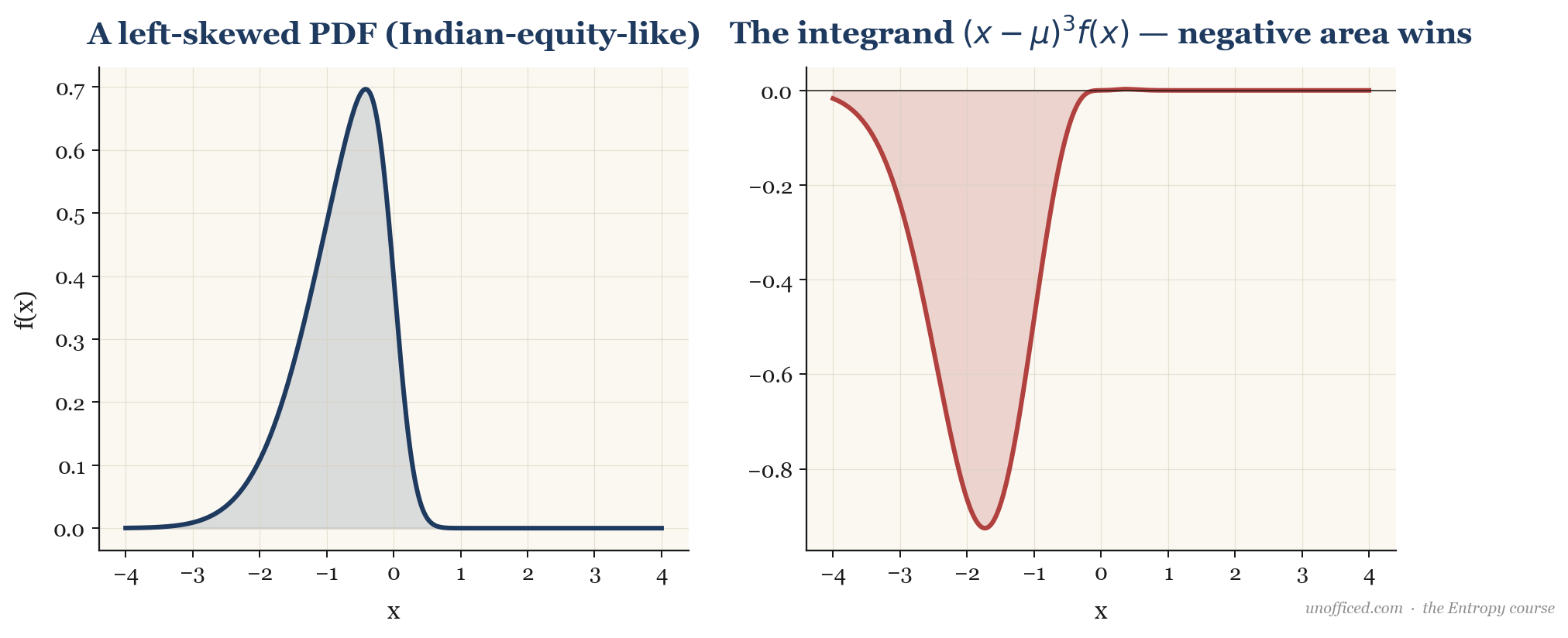
The third central moment is the expectation of the cubed deviations from the mean. It measures the weighted average of the asymmetry of the distribution.
The integrand gives large positive weight to outcomes far above the mean and large negative weight to outcomes far below the mean. If the negative values dominate, the integral (and thus the skewness) will be negative.
Standardizing this moment by dividing by makes it a dimensionless quantity, allowing us to compare the skewness of different distributions regardless of their scale.
The value of tells us the direction and degree of the asymmetry:
- : The distribution is perfectly symmetric. The tails on either side of the mean are of equal length and weight. A Gaussian (Normal) distribution is the canonical example.
- : The distribution is positively skewed or right-skewed. The right tail is longer and fatter than the left tail. This implies a higher probability of large positive outcomes. In trading terms, this means frequent small losses and a few very large gains (e.g., venture capital or trend-following strategies).
- .
The standard deviation is approximately Rs. 38,400.
The third moment is dominated by the large negative outcomes: the cubed deviation for the loss is , while for the gain it is . Even though there are far more gains, the sheer magnitude of the cubed loss term ensures the expected value of the cubed deviations will be large and negative. The calculated skewness for this distribution is approximately -3.6, indicating extreme negative skew.
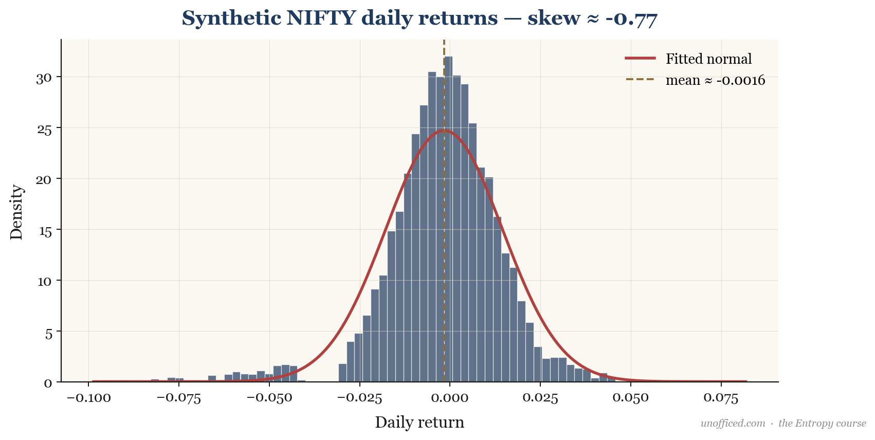
Skewness in Indian Equity Returns
When we analyse the historical daily log returns of broad market indices like the NIFTY 50 or BANKNIFTY, we consistently find evidence of negative skewness. Empirically, the skewness of NIFTY 50 daily returns typically falls in the range of -0.3 to -0.6. For the more volatile BANKNIFTY, the skew is often more pronounced, ranging from -0.4 to -0.8.
Why does this happen? A primary explanation, first proposed by Fischer Black in 1976, is the leverage effect. As a company’s stock price falls, its market capitalization (Equity) decreases while its debt level remains fixed. This automatically increases the company’s financial leverage (Debt-to-Equity ratio). Higher leverage makes the stock riskier, implying that future cash flows are discounted at a higher rate, which in turn leads to an increase in its perceived volatility. This feedback loop—falling prices causing higher volatility—can create disproportionately large down-moves compared to up-moves, resulting in a negatively skewed return distribution.
Why a Trader Cares About Skewness
Mean and standard deviation are insufficient for risk management. Two trading strategies can have identical means and volatilities but completely different risk profiles due to skewness.
Many popular options-selling strategies, such as writing covered calls or shorting straddles and strangles, are classic examples of generating a negatively skewed return profile. The trader collects a regular premium (frequent small gains), but is exposed to unlimited or very large losses if the underlying asset makes a sudden, sharp move against their position, especially over a weekend (gap risk). The median trade is profitable, but the mean return is dominated by the rare, deep losses in the left tail.
Sample Estimators for Skewness
In practice, we don’t know the true parameters of the distribution. We must estimate skewness from a sample of data (e.g., a time series of daily returns). The simplest sample skewness estimator, , is calculated as:
Here, is the sample mean and is the sample standard deviation. This is the basic Fisher-Pearson coefficient of skewness. However, this estimator is biased, especially for small sample sizes. Most statistical software packages use a bias-corrected estimator, :
This adjustment factor corrects for the downward bias of the sample third moment. It’s crucial to know which estimator your software is using.
A common variant, Pearson’s second skewness coefficient, replaces the mode with the median, as the mode can be difficult to estimate robustly for continuous data:
This measure is less sensitive to extreme tail events but provides a quick gauge of asymmetry based on the relative positions of the central tendency measures.
Statistical Tests for Skewness
To formally test if the skewness of a sample is significantly different from zero (the value for a normal distribution), several statistical tests are available. The D’Agostino’s K-squared test is specifically designed to test for departures from normality due to skewness. More commonly, skewness is tested jointly with kurtosis in a composite test for normality, such as the Jarque-Bera test. A significant p-value from these tests provides statistical evidence that the return distribution is not symmetric, warranting a closer look at its tail properties.
Summary
Skewness is an indispensable tool for financial risk analysis. It moves our understanding of a return distribution beyond simple averages and volatility into the critical domain of asymmetry.
- Skewness measures the asymmetry of a distribution around its mean, calculated as the third standardized moment.
- Positive skew () implies a longer right tail (potential for large gains), while negative skew () and an understanding of bias correction.
While skewness tells us about the direction of asymmetry, it doesn’t describe the “fatness” of the tails on both sides simultaneously. A distribution could be symmetric but still have a much higher probability of extreme events than a normal distribution. To measure this property, known as tail risk, we turn to the fourth moment: Kurtosis.
Further Reading
- Ross, Sheldon M. A First Course in Probability. Pearson. (A foundational text on probability theory that covers moments of a distribution.)
- Taleb, Nassim Nicholas. The Black Swan: The Impact of the Highly Improbable. Random House. (A philosophical and practical exploration of the impact of rare, extreme events, which are the drivers of skewness.)
- Wilmott, Paul. Paul Wilmott on Quantitative Finance. John Wiley & Sons. (A comprehensive guide for practitioners that frequently discusses the practical implications of skewness and other higher moments in derivatives pricing and risk management.)