Log-Normal Distribution

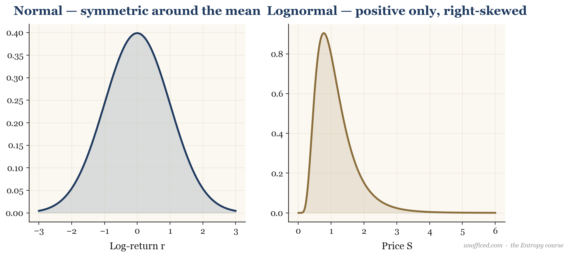
A lognormal distribution arises when the natural logarithm of a variable follows a normal distribution. In finance, this distribution is fundamental because the standard model for stock price dynamics, Geometric Brownian Motion (GBM), implies that future stock prices are lognormally distributed. This is a direct consequence of stock returns compounding over time. Unlike a normal distribution, a lognormal distribution only takes positive values, which accurately reflects the fact that a stock’s price cannot be negative, a feature essential for realistic market modelling.

Rigorous Definition and Derivation

A continuous random variable X is said to have a lognormal distribution if its natural logarithm, Y = ln(X), is normally distributed. If , where is the mean and is the variance of the log-variable, then X follows a lognormal distribution, denoted .

The probability density function (PDF) for X can be derived from the PDF of the normal variable Y using the change of variables technique. Let be the PDF of Y:

Given , we have and the derivative (the Jacobian of the transformation) is . The PDF of X, , is then :

Visually, the lognormal distribution is skewed to the right, in contrast to the symmetric bell curve of a normal distribution. This positive skewness means that while most outcomes are clustered at the lower end, there is a small probability of extremely high values—a “long tail” to the right.

Why Stock Prices are Modelled as Lognormal

The cornerstone model for stock price movement is Geometric Brownian Motion (GBM). It describes the change in a stock’s price, , as a combination of a deterministic drift (, the expected return) and a random shock (, volatility scaled by a Wiener process, which represents a random walk).

The stochastic differential equation (SDE) for GBM is:

This equation states that the incremental change in price () is the sum of a drift component proportional to the current price and a random component also proportional to the current price. This proportionality ensures that the model is realistic: a Rs. 10 change is more significant for a Rs. 100 stock than for a Rs. 3,000 stock. The model works with percentage returns, which are scale-free.

To solve for , we cannot use standard calculus because of the stochastic term . We must use Itô’s calculus. Applying Itô’s lemma to the function , we find the dynamics of the log-price:

Integrating from 0 to T gives the solution:

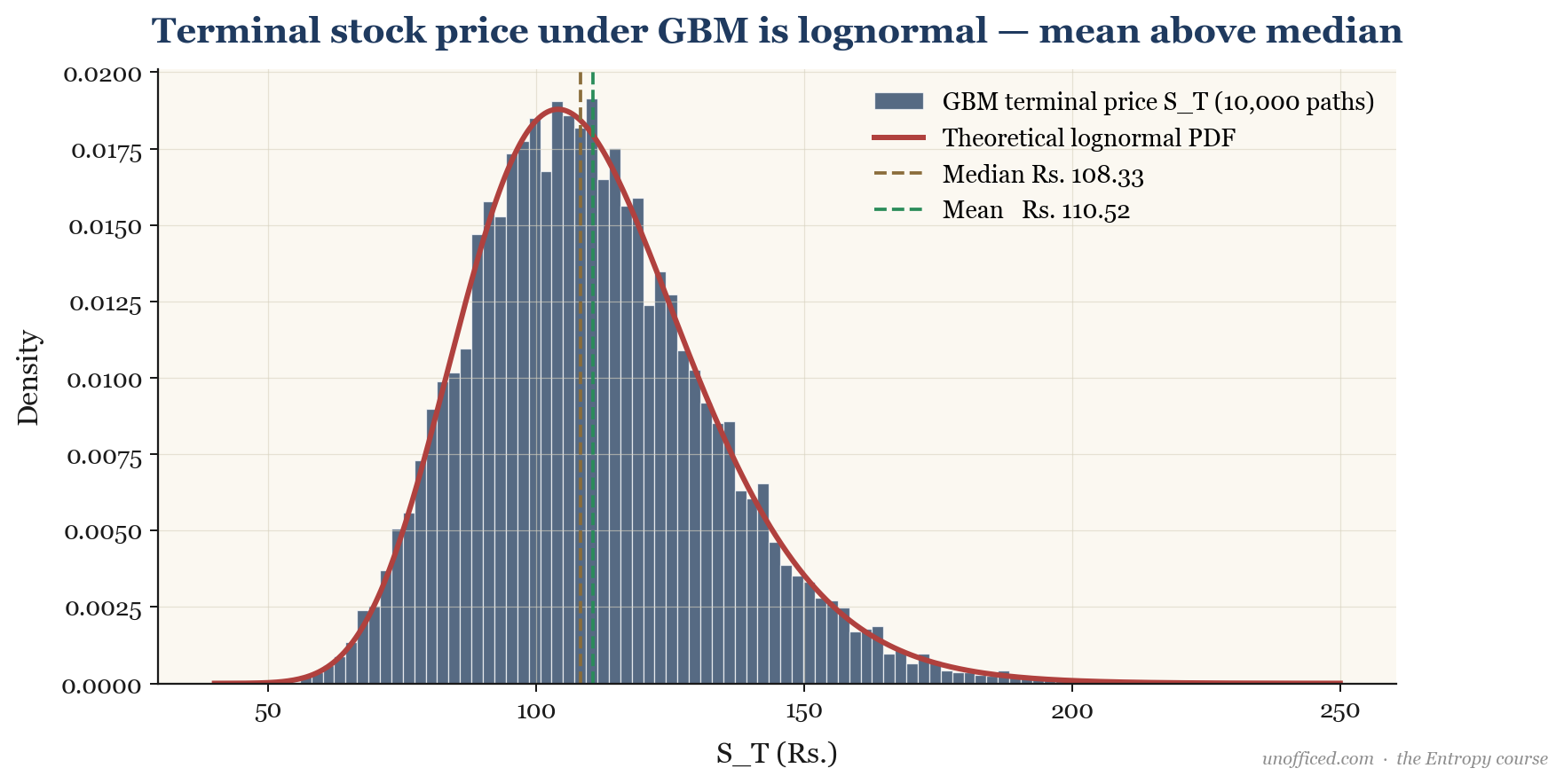
Since and , the term is normally distributed with mean 0 and variance . The right-hand side is a constant (), a deterministic term, and a normally distributed random term. This proves that the log-price, , is normally distributed. Consequently, the future price itself, , must be lognormally distributed.

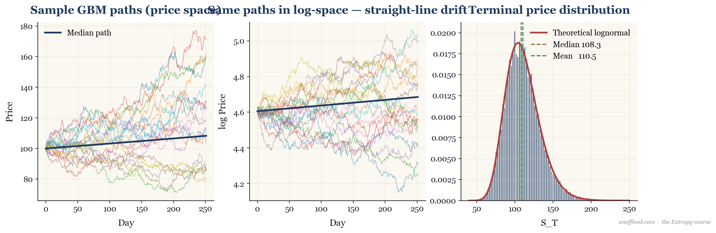
The plot below shows twenty possible price paths simulated using the GBM model. The distribution of prices at any future point in time is lognormal.

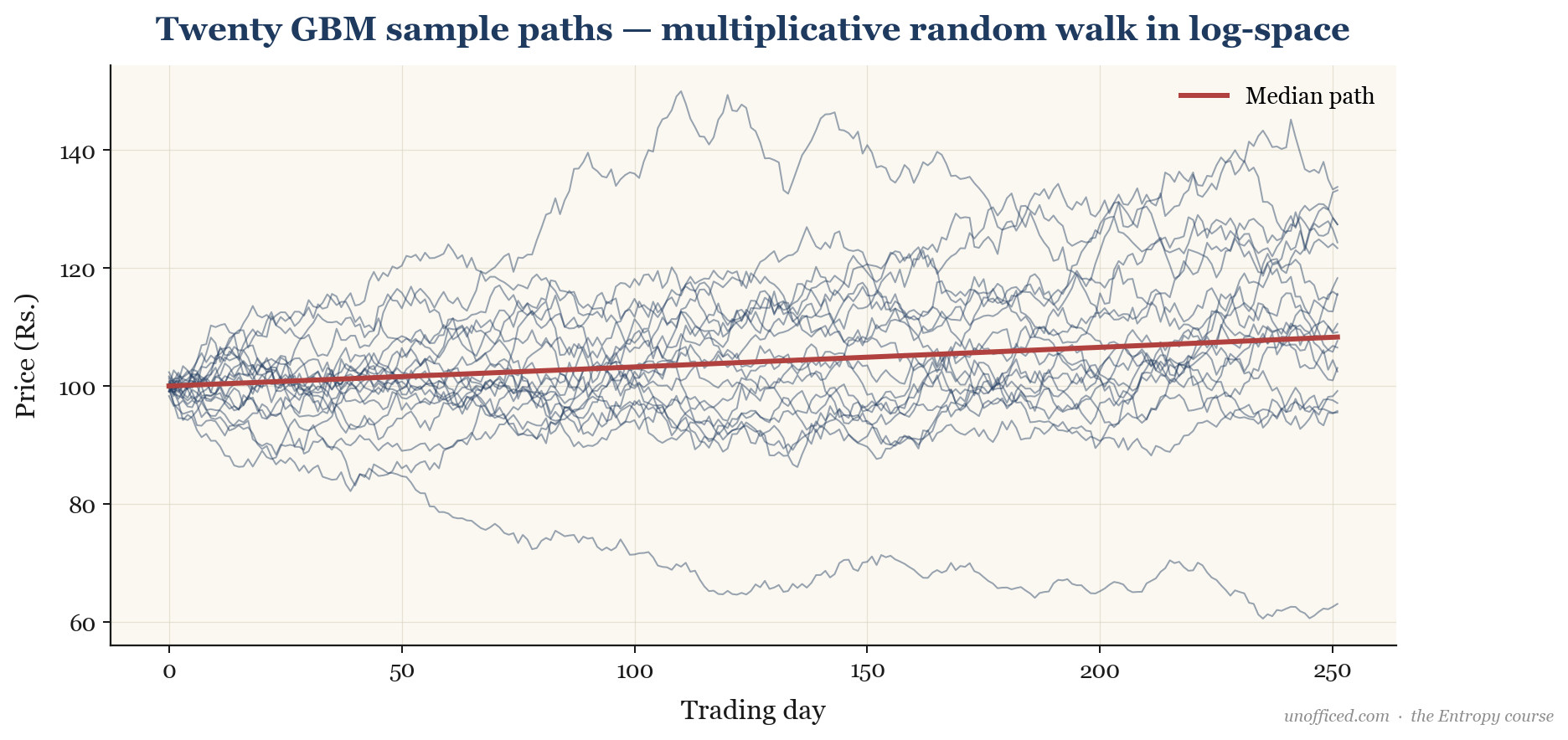
What this means for a trader: Your portfolio’s value over time is not a simple linear projection. High volatility () actively works against your compounded growth rate. Two assets with the same expected return () but different volatilities will have vastly different long-term outcomes. The less volatile asset will almost always have a higher terminal value, even if they share the same average arithmetic return.

Moments and Characteristics

For a lognormal variable X where , the key statistical moments can be derived using the moment generating function (MGF) of the underlying normal variable. The MGF of is . The k-th moment of X is .

• Mean (E[X]): Set k=1.
• Variance (Var(X)):
• Median: The median corresponds to the point where the cumulative probability is 0.5. For the underlying normal distribution, this is at the mean . Thus, the median of X is .

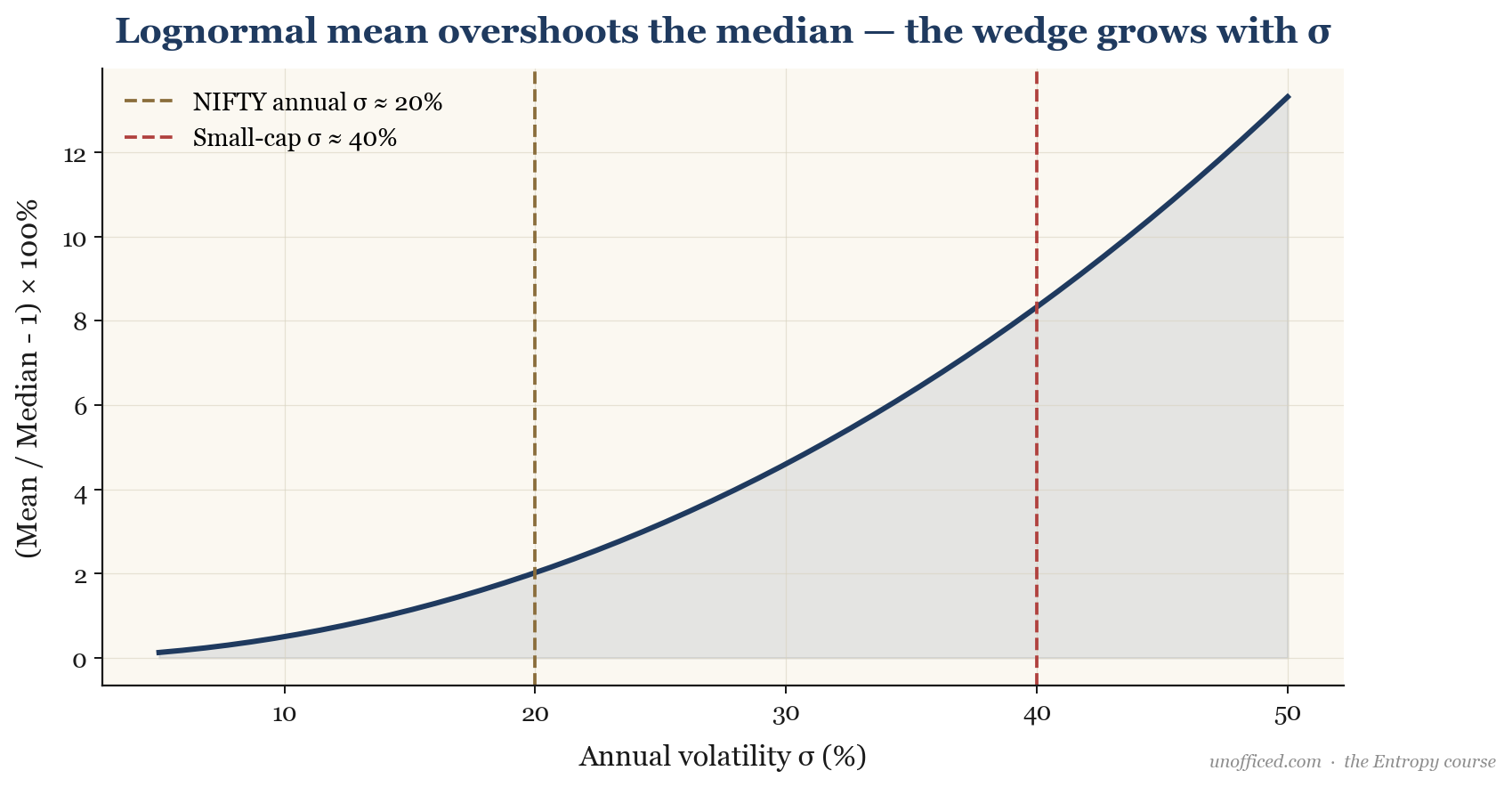
A crucial feature is that the mean is always greater than the median, as for any . This is a direct result of the positive skewness; the possibility of rare, extremely high outcomes pulls the average (mean) above the typical midpoint (median).

Worked Example: NIFTY 50 CAGR vs Arithmetic Mean

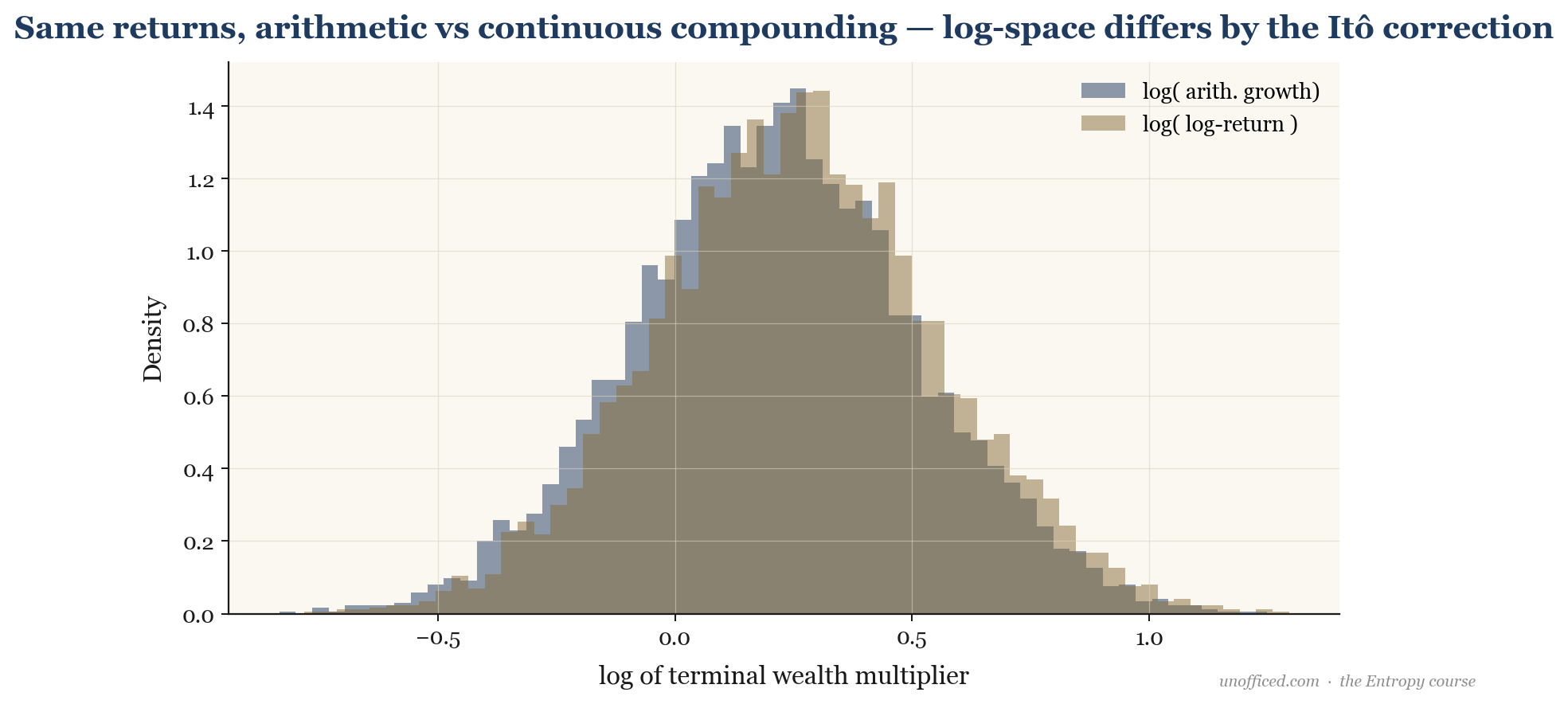
Let’s look at the historical performance of the NIFTY 50 index. Over a typical 10-year period, the average of the annual returns (the arithmetic mean) might be around 14%. However, the actual Compound Annual Growth Rate (CAGR), which represents the geometric mean, is often closer to 12%. Where does the 2% difference go?

This “lost” return is the volatility drag. If we model the NIFTY’s log-returns as being approximately normal, we can relate the two:
.
With an annual volatility of around 20% (0.20), the drag is , or 2%. This perfectly explains the discrepancy. An investor’s actual wealth compounds at the geometric rate, not the higher arithmetic one.

Worked Example: Projecting ICICI Bank Share Price

Suppose ICICI Bank stock ([`ICICIBANK`]) is trading at Rs. 1,200 on the NSE. An analyst estimates its annual expected return () to be 18% and its annual volatility () to be 30%. What are the expected mean and median prices after one year ()?

First, we find the parameters for the log-price :

• The mean of the log-price is the continuously compounded expected return: .
• The variance of the log-price is .

Now, we can calculate the key price levels for :

• Median Terminal Price (most probable outcome) =
• Mean Terminal Price (expected value) =

After one year, the most likely single outcome (median) is a price of Rs. 1,373.34. However, the average of all possible outcomes (the mean) is Rs. 1,436.45. The difference of Rs. 63.11 is the “volatility bonus” paid to the mean by the skewed distribution’s long right tail.

Implication for Risk Management and Option Pricing

The lognormal model is the mathematical bedrock of modern finance. Its most famous application is in the Black-Scholes-Merton (BSM) model for pricing European options. The BSM formula assumes that the underlying asset’s price at the option’s expiry follows a lognormal distribution. This assumption is what allows for a closed-form solution for option prices.

Furthermore, the lognormal property is critical for portfolio management. For example, the Kelly Criterion, a formula for optimal bet sizing to maximize long-run capital growth, has versions specifically adapted for lognormally distributed returns (e.g., by Ed Thorp). It uses the mean and variance of log-returns ( and ) to determine the optimal fraction of capital to allocate to a risky asset.

What this means for a trader: Understanding the lognormal assumption helps you know when your tools will work. Using BSM to price NIFTY options on a normal trading day is appropriate. Using it to price options on an illiquid penny stock ahead of a court ruling is a recipe for disaster, as the real distribution will have fatter tails and more jump risk than the lognormal model allows.

A Note on Bollinger Bands

Bollinger Bands are constructed by adding and subtracting a multiple of the rolling standard deviation from a moving average of prices. This implicitly assumes that prices are roughly normally (symmetrically) distributed around their mean. However, as we’ve established, prices are lognormally distributed and skewed.

Summary

The lognormal distribution is a more realistic and powerful model for stock prices than the normal distribution. Here are the key takeaways for a quantitative trader:

• It naturally arises from the compounding of returns, as formalised by the Geometric Brownian Motion model, and guarantees positive prices.
• The distribution is positively skewed. The mean (expected value) is greater than the median (most likely outcome), and this gap grows exponentially with volatility.
• Your portfolio grows at the geometric rate (), not the arithmetic rate (). High volatility is a direct drag on your compounded returns.
• This distribution is the core assumption of the Black-Scholes-Merton option pricing model and has applications in advanced risk management techniques like the Kelly Criterion.
• It is a good model for liquid, large-cap assets but fails for assets prone to sudden, large jumps.

Further Reading

1. The Lognormal Distribution by E. L. Crow and K. Shimizu. A comprehensive statistical reference on the distribution itself.
2. Options, Futures, and Other Derivatives by John C. Hull. The chapter on Wiener processes and Itô’s Lemma provides a very accessible derivation of the GBM model.
3. The Kelly Capital Growth Investment Criterion edited by L. C. MacLean, E. O. Thorp, and W. T. Ziemba. Contains several papers, including Thorp’s, on applying the criterion under lognormal return assumptions.
4. Quantitative Finance by Paul Wilmott. Provides a trader-focused, practical guide to these concepts.