Standard Deviations

Standard deviation is a statistical measure that quantifies the dispersion of a set of values around their mean. For a trader, it provides a direct answer to a critical question: how much does an instrument’s price typically swing? A low standard deviation implies price action is tight and constrained, while a high standard deviation suggests wide, volatile fluctuations. It is the foundational measure of price volatility, the very heartbeat of the market.
What is Standard Deviation?
Standard deviation is the square root of variance. Variance, in turn, measures the average of the squared differences from the mean. For a theoretical population of all possible outcomes, the variance () is the expected value of the squared deviation of a random variable () from its population mean ().
The standard deviation () is simply the square root of this value. The units of standard deviation are the same as the units of the data itself (e.g., points for NIFTY, or percentage for returns), making it more interpretable than variance.
In practice, traders don’t have access to the entire population of returns. We work with a sample of data, such as the last 20 closing prices. To estimate the population’s standard deviation from a sample, we use the sample variance formula:
Here, is the sample mean (the average of our data points) and is the number of data points in the sample. The resulting sample standard deviation ( or ) is the square root of the sample variance.
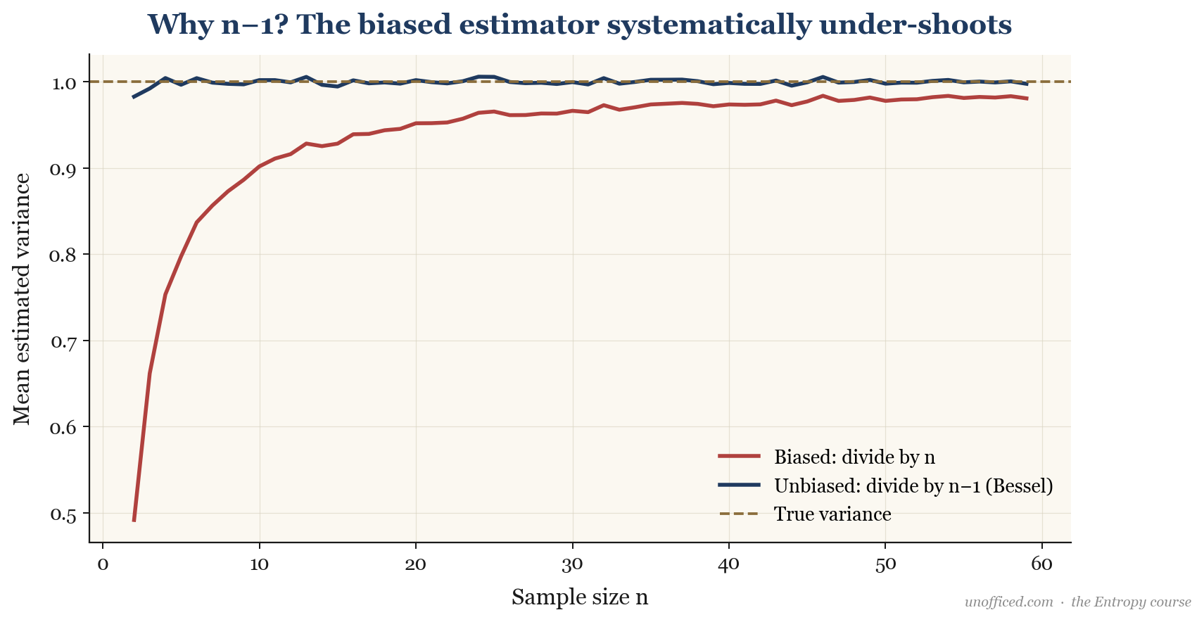
Formal Proof of Bessel’s Correction
Why does dividing by give an unbiased estimate? We want to show that the expected value of the sample variance equals the population variance . That is, .
Starting with the numerator, the sum of squared deviations:
Since , it follows that . Substituting this in:
Now, let’s take the expectation. We use the facts that and .
So, the expected value of the sum of squared deviations is . To get an unbiased estimator for , we must therefore divide by :
This proves that the sample variance formula with is indeed an unbiased estimator of the population variance.
The Empirical Rule vs. Chebyshev’s Inequality
If we can assume that asset returns follow a Normal Distribution (a symmetric bell curve), standard deviation provides a powerful framework for estimating the probability of price movements. This is often called the empirical rule.
- Approximately 68.3% of all values lie within 1 standard deviation of the mean ().
- Approximately 95.4% of all values lie within 2 standard deviations of the mean ().
- Approximately 99.7% of all values lie within 3 standard deviations of the mean ().
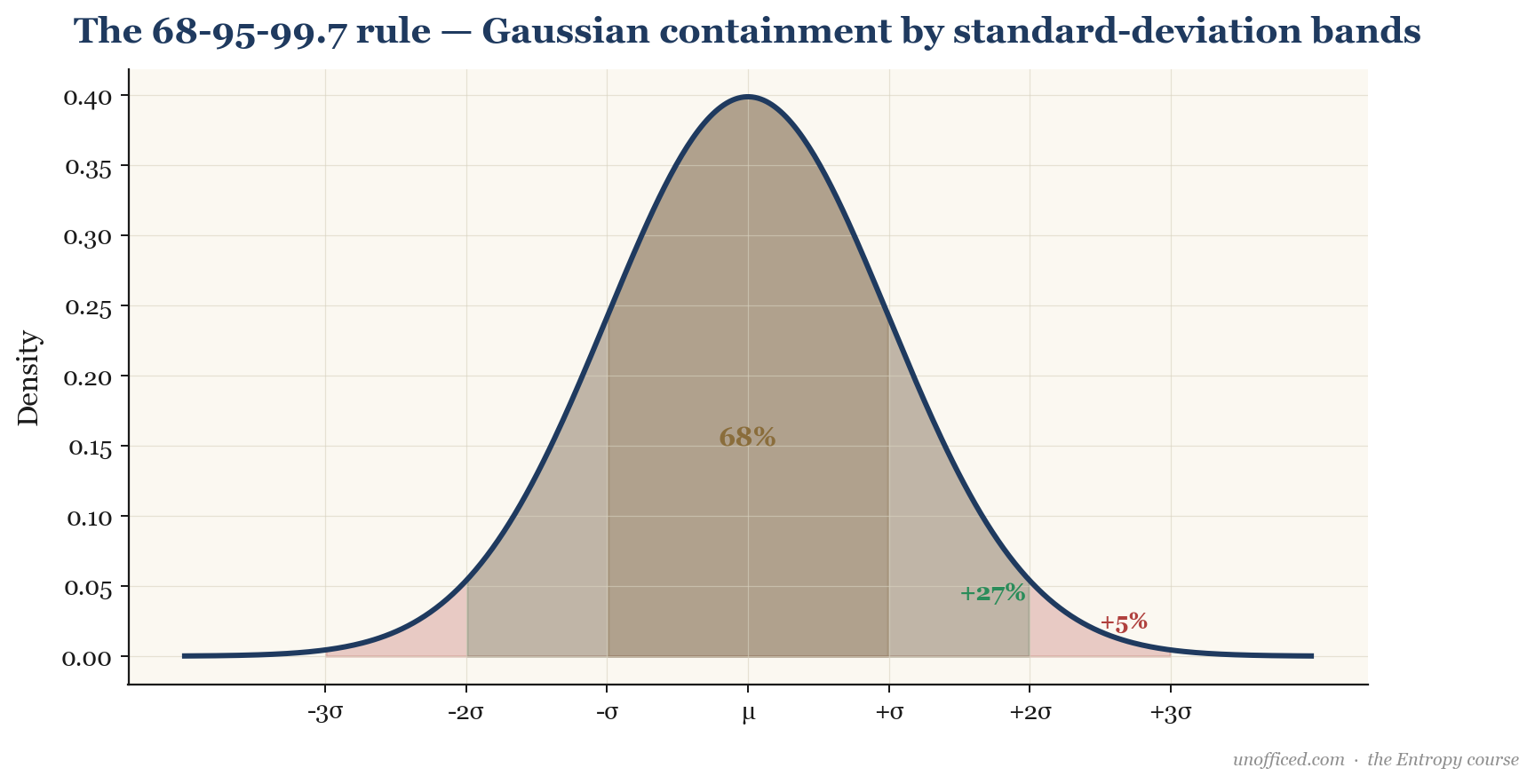
This is the statistical foundation for Bollinger Bands, which are typically drawn at 2 standard deviations above and below a central moving average. A price touching the bands is a 2-sigma event, which is expected to occur only about 5% of the time under the crucial assumption of normality.
A Universal Backstop: Chebyshev’s Inequality
But what if we can’t assume returns are normal? Financial returns are notoriously non-normal. Is standard deviation still useful? Yes. Chebyshev’s inequality gives us a “worst-case” bound on probabilities that holds for any distribution, regardless of its shape.
It states that for any random variable with a finite mean and finite non-zero variance , for any real number , the probability that will be at least standard deviations away from the mean is no more than .
Let’s compare this to the empirical rule:
| Deviation | Max Probability Outside (Chebyshev) | Min Probability Inside (Chebyshev) | Probability Inside (Normal) |
|---|---|---|---|
| 95.4% | |||
| 99.7% | |||
| 99.99% |
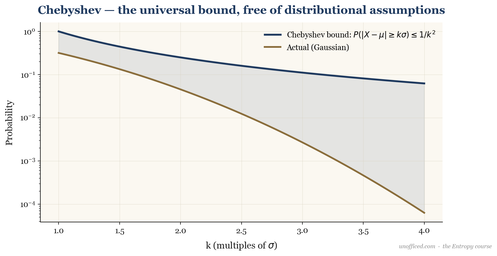
What this means for a trader: Chebyshev’s inequality is a crucial piece of risk management wisdom. It reminds us that tail events can be more common than a simple bell-curve model would suggest. While the 68-95-99.7 rule is a useful guidepost, a robust risk model must account for the possibility of non-normal, “fat-tailed” distributions where 3- and 4-sigma events are not as rare as we’d like.
Volatility in Practice
Standard deviation quantifies the character of price action. Consider three different time series below. All have the same mean return (zero), but their standard deviations are vastly different.
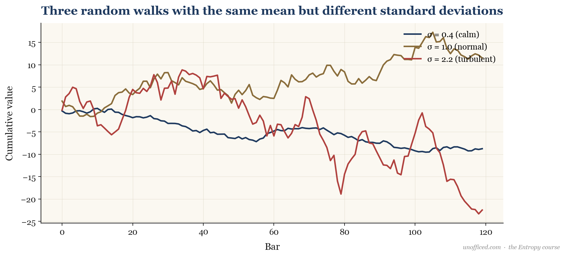
The series with the highest standard deviation (2.2) exhibits the wildest swings, representing a highly volatile asset like a small-cap stock after an earnings surprise. The one with the lowest SD (0.4) is far more placid, perhaps like a large blue-chip stock such as HDFC Bank in a quiet market. This visualises how a single number can describe the magnitude of an asset’s price fluctuations.
Worked Example: NIFTY Closes
Let’s compute the sample standard deviation for five hypothetical NIFTY 50 closing prices: 21,540, 21,605, 21,520, 21,610, and 21,655.
1. Calculate the mean ():
2. Calculate squared deviations from the mean:
| Close () | Deviation () | Squared Deviation () |
|---|---|---|
| 21,540 | -46 | 2,116 |
| 21,605 | 19 | 361 |
| 21,520 | -66 | 4,356 |
| 21,610 | 24 | 576 |
| 21,655 | 69 | 4,761 |
3. Sum the squared deviations:
4. Calculate the sample variance ():
5. Calculate the sample standard deviation ():
The standard deviation for this five-day period is approximately 55.16 NIFTY points. This number suggests that a typical daily price swing during this period was around 55 points from the average.
Rolling Standard Deviation
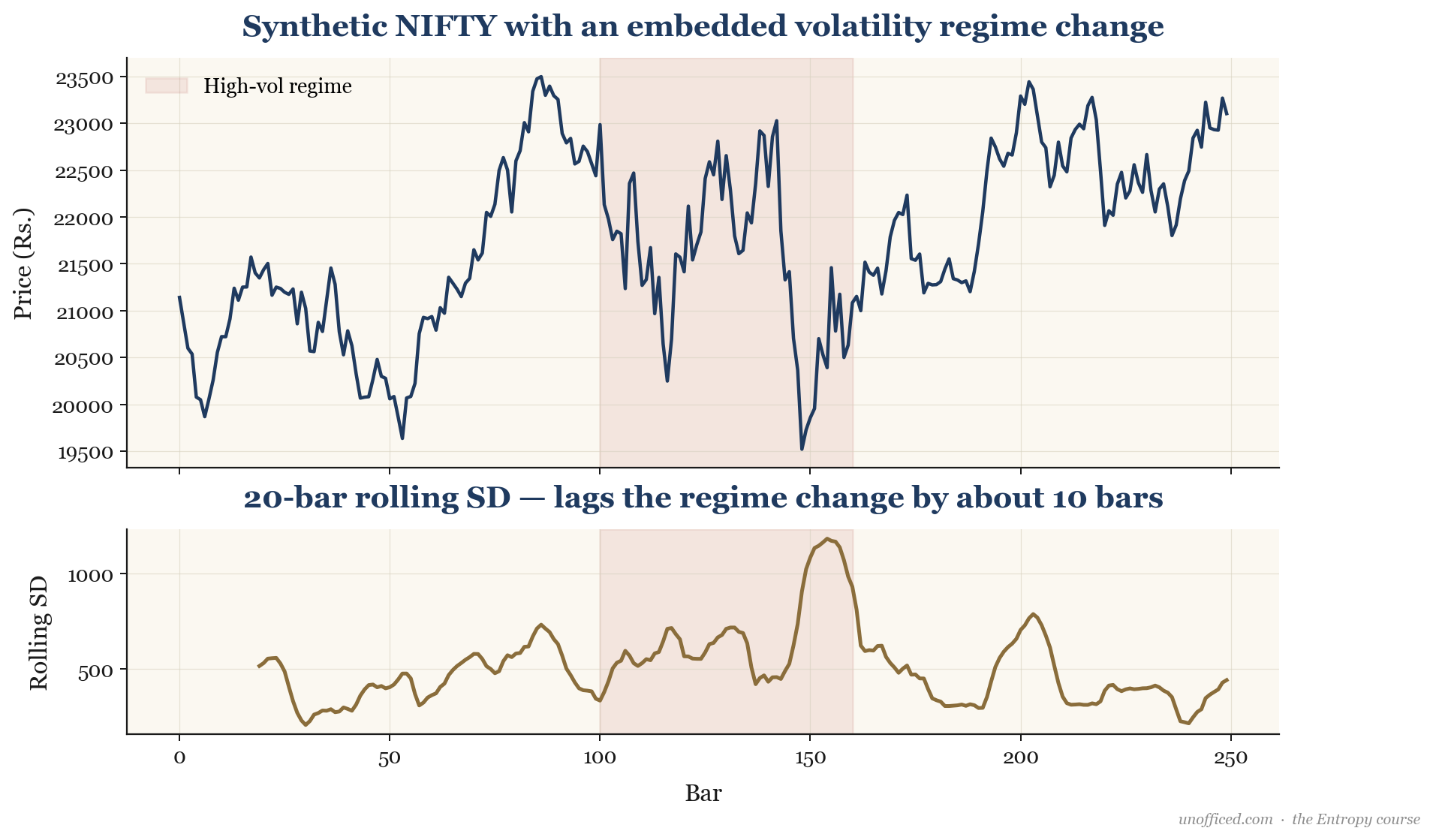
In trading, we are rarely interested in the standard deviation of a fixed dataset. We need to know how volatility is evolving over time. For this, we use a rolling standard deviation, which computes the SD over a moving window of the most recent n periods (e.g., 20 bars).
This is precisely what a Bollinger Band indicator does. It calculates a 20-period moving average and then adds and subtracts 2 times the 20-period rolling standard deviation.
A crucial feature of any rolling estimator is that it introduces lag. As the chart shows, when the market transitions from a low-volatility to a high-volatility regime, the rolling SD indicator takes time to “catch up.” The lag is typically around half the length of the lookback window (). This is why Bollinger Band “squeezes” often give way to powerful breakouts; the bands are playing catch-up to a new volatility reality.
Window 1 (Days 1-4): Prices are 3410, 3420, 3415, 3430. Mean is 3418.75. SD is .
Window 2 (Days 2-5): Prices are 3420, 3415, 3430, 3450. Mean is 3428.75. SD is . The volatility has increased.
Window 3 (Days 3-6): Prices are 3415, 3430, 3450, 3440. Mean is 3433.75. SD is . Volatility remains elevated.
This is how a rolling standard deviation indicator on a charting platform would compute its values bar-by-bar.
Annualising Volatility & Standard Error
You will often hear volatility quoted as an annualised percentage (e.g., “INDIA VIX is at 15”). To convert a daily standard deviation to an annual one, we scale it by the square root of the number of trading days in a year, which is approximately 252 for Indian markets.
This square-root-of-time rule stems from the properties of variances of independent random variables. If daily returns are independent with variance , then the variance over days is . The standard deviation is the square root, hence .
For example, if RELIANCE has a daily standard deviation of returns of 1.5%, its annualised volatility would be .
The Standard Error of the Mean
A related and critical concept is the standard error of the sample mean. If we take many samples from a population and calculate the mean of each, those sample means will themselves form a distribution. The standard deviation of this distribution is the standard error (SE). It tells us how precisely our sample mean estimates the true population mean.
For a sample of size from a population with standard deviation , the variance of the sample mean is:
The standard error of the mean is the square root of this:
What this means for a trader: The standard error formula is profound. It shows that our confidence in an estimated edge (mean return) increases with the square root of the number of trades. To double the precision of our estimated mean, we need to quadruple the sample size. This is a fundamental law of statistical trading: reliable estimates require a large amount of data.
The Achilles’ Heel of SD: Robust Statistics
Standard deviation’s greatest weakness is its extreme sensitivity to outliers. The formula squares the deviations, meaning a single large outlier can dramatically inflate the final value. For example, a 10-sigma event contributes times more to the variance calculation than a 1-sigma event. In financial markets, which are prone to sudden gaps and crashes (fat tails), standard deviation can often be misleading.
Median Absolute Deviation (MAD)
A more robust measure of dispersion is the Median Absolute Deviation (MAD). It is the median of the absolute differences between the data points and their median.
To make MAD comparable to standard deviation for Normally distributed data, we scale it by a constant factor.
The constant 1.4826 is approximately , where is the inverse of the cumulative distribution function for the standard normal distribution.
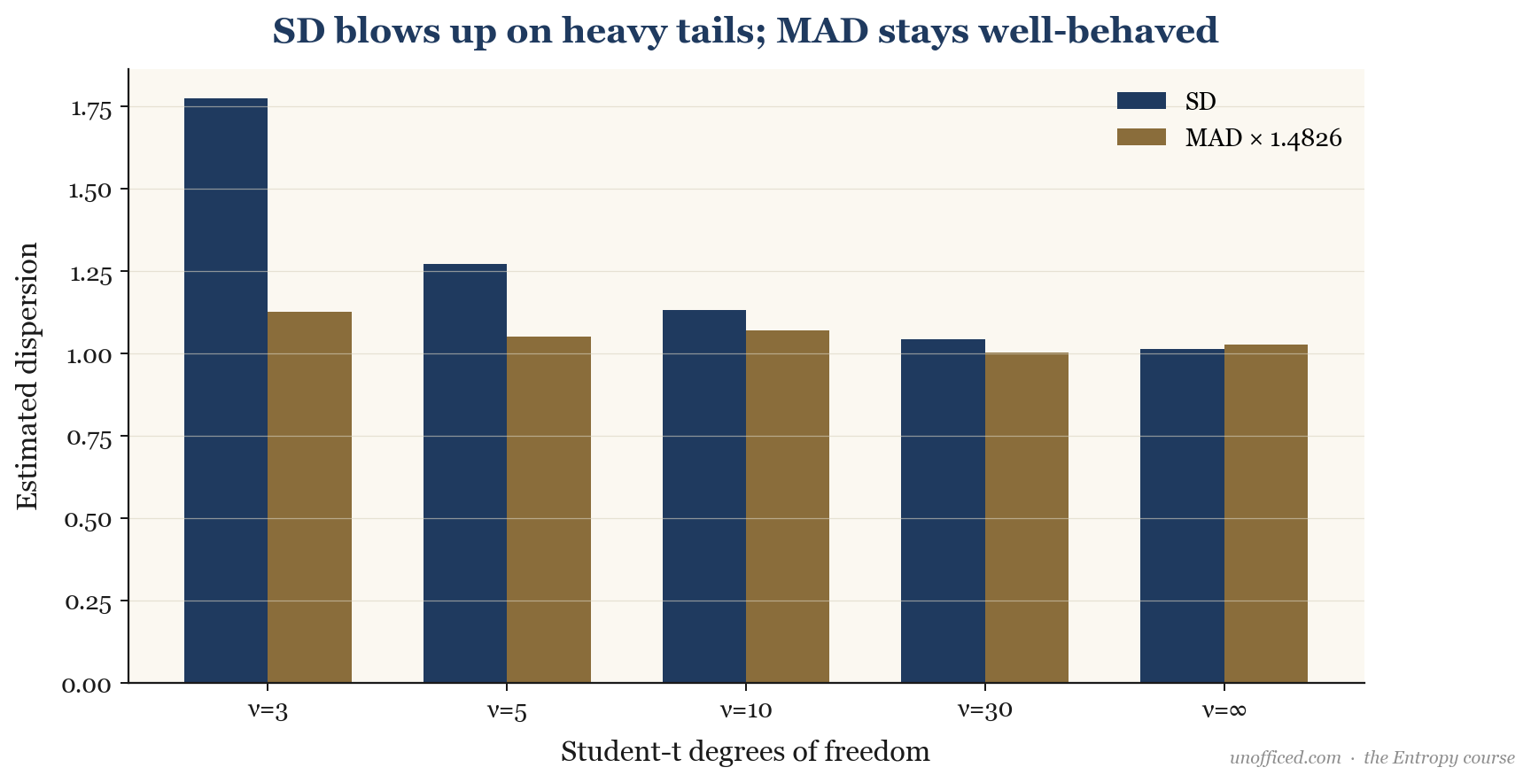
The image above shows a price series with a sudden jump. The standard deviation, calculated over the whole period, is massively skewed by this single event. The MAD, however, is barely affected, providing a more stable and representative measure of the ‘typical’ dispersion, ignoring the outlier.
What this means for a trader: When your risk model uses standard deviation, you are implicitly making a bet that huge outliers won’t happen, or will be so rare that they don’t matter. History shows this is a bad bet. Using a robust measure like MAD for setting stop-losses, position sizing, or value-at-risk (VaR) calculations can provide a more conservative and realistic assessment of risk, especially in markets prone to extreme moves like individual stocks or cryptocurrencies.
Further Reading
To deepen your understanding of these foundational statistical concepts, the following resources are invaluable:
- A First Course in Probability by Sheldon Ross: An essential and accessible introduction to the fundamental principles of probability theory that underpin all of statistics.
- Time Series Analysis by James D. Hamilton: The canonical graduate-level textbook on time series models, including detailed treatments of concepts like volatility clustering and GARCH models.
- The Black Swan: The Impact of the Highly Improbable by Nassim Nicholas Taleb: A philosophical and qualitative exploration of the importance of fat tails, outliers, and the limits of standard statistical models in finance.
- Paul Wilmott on Quantitative Finance by Paul Wilmott: A comprehensive and practical guide covering many aspects of quantitative finance, with clear explanations of how statistical measures are used in pricing and risk management.
Summary
- Standard deviation (SD) is the most common measure of price volatility, quantifying dispersion around the mean.
- For a sample of data, we use the Bessel-corrected formula (dividing by n-1) to get an unbiased estimate of the true population variance.
- The 68-95-99.7 rule is a useful heuristic but relies on the often-flawed assumption of Normal distributions. Chebyshev’s inequality provides a weaker but universal bound.
- Technical indicators use a rolling SD to track how volatility changes over time, but this introduces a response lag of approximately n/2 periods.
- Daily SD can be annualised by multiplying by , but one must be aware of the flawed i.i.d. assumption this makes.
- Standard deviation is highly sensitive to outliers. Robust alternatives like Median Absolute Deviation (MAD) provide a more stable measure of dispersion in the presence of fat tails.
While standard deviation tells us about the magnitude of price swings, it doesn’t describe the shape or symmetry of the return distribution. Two assets can have the same SD but behave very differently. To understand that, we need to look at the next moments of the distribution: skewness and kurtosis.