Probability Distribution

A probability distribution is a statistical function that describes all the possible values and likelihoods that a random variable can take within a given range.

There are many different types of probability distributions. One of them is the normal distribution. A probability distribution has a number of factors which is used to describe it – mean, standard deviation, skewness, kurtosis.

We are already aware of mean and standard deviation. But let’s get inside of kurtosis and skewness.

Dispersion

Standard deviation is a measure of the dispersion of a set of data from its mean. If the data points are further from the mean, there is the higher deviation from the data set.
Dispersion is a statistical term describing the size of the range of values expected for a particular variable.
Like, beta is a familiar risk measurement which measures the dispersion of a security’s returns relative to a particular benchmark or market index. You can see how it is calculated in more details here.

Normal Distribution

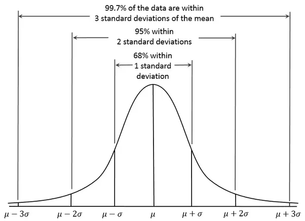
The standard normal distribution or normal distribution is symmetrical data distribution where most of the results lie near the mean.

A standard normal distribution is divided symmetrically using mean of the distribution. ( interpret it as the average of the data set)

Where:

Mu is mean of the distribution
Sigma is the standard deviation

If you consider settings of Bollinger Bands as following –

Period – 20
Standard Deviations – 2
Moving Average Type – Simple

Then it means if we take last 20 price points and plot a line with their average; then it is the median Bollinger.

Here is how it is calculated if you abide by the settings of our 2 SD Bollinger –

Middle Band = 20-day exponential moving average (EMA)
Upper Band = 20-day EMA + (20-day standard deviation of price x 2)
Lower Band = 20-day EMA – (20-day standard deviation of price x 2)

Now if you closely look at the formulas, we can say that 95% prices of a scrip from stock market stay within Bollinger bands of 2 standard deviations.

And, 68% prices of a scrip from stock market stays within Bollinger bands of 1 standard deviation.

Isn’t that amazing?

But we are assuming here that stock market prices follow a standard normal distribution, do they?

Q. Let us take an example of 1 SD Bollinger band. The upper and lower bands also keep on changing with the mean. So according to the theory, the price will be between upper and lower bands 68% of the times.

A. What you said is right. 68% of data should fall within one standard deviation and that roughly 95% should fall within two standard deviations considering normal distribution but Bollinger bands work best in case of the ranged market and fails in case of a trending market. There are some cases where Bollinger assumption fails (for 68% and 95%) because it’s not actually a perfectly normal distribution. If we map with the historical price charts for Nifty the numbers for 1SD and 2SD come out closer to 65% and 90%.

Q. Then how BRS is working in trending market?

A. BRS actually follows a ranged market. We’re here actually trading here in the range of 1 SD to 2 SD. It tells out that the stock has broken one range and is ready to move another range. Now how you trade it and whether you can ride it even if it crosses 2 SD depends on your exit strategy.

Now let’s say Infibeam rose from 1000 to 1010 on 1 day. On a linear scale, its 10 points on the chart but on a logarithmic price scale its % (or fraction) so its 1% change.

Now let’s say another day Infibeam rose from 1010 to 1020. On a linear scale it’s still 10 points on the chart but on a logarithmic price scale its % (or fraction) so it’s 0.99% change. Linear scale fails to consider the relative change, hence logarithmic scale is used.

Q. So can it be concluded that the BRS strategy has no mathematical fact backing it? Is it just a matter of trader’s intuition and experience?

A. Completely false. It’s based completely on a mathematical fact. The moment the stock moves out of 1 SD it’s actually creating a newer band for itself and the probability of it to follow the same trend is very high.

Q. Shouldn’t the stock be more inclined to come back to the 65% bracket, and the break out of 1SD being a case of remaining 35%?

A. 80% of the time (statistically backtested) market trades in a range and the moment price moves in the 1 SD and 2 SD upper band away from mean (i.e median Bollinger) it moves into a buy zone and vice versa with lower bands.

Here comes something called conditional probability. It’s not just a normal case of 65% vs 35% but a case of Probability( it remaining above 1 SD | it has crossed 1 SD) or Probability of staying above 1 SD given it has already crossed 1 SD.

Mean, Median, Mode

The mean is the average of all numbers.

The statistical median is the middle number in a sequence of numbers. If there is an even set of numbers, average the two middle numbers.

The mode is the number that occurs most often within a set of numbers. Mode helps identify the most common or frequent occurrence of a characteristic. It is possible to have two modes (bimodal), three modes (trimodal) or more modes within larger sets of numbers.