Continuous Compounding

In finance, compounding is the engine of growth. While most are familiar with periodic compounding (monthly, quarterly, or annually), there is a more powerful, theoretical limit: continuous compounding. Here, interest is calculated and added to the principal not just daily or hourly, but at every infinitesimal instant.
For traders and quants, this is not just a mathematical curiosity. Continuous compounding and its cousin, the logarithmic return, form the bedrock of how we model and analyse asset price movements. They are the natural language of financial markets, essential for everything from risk management to pricing the most complex derivatives.
From Periodic to Continuous Compounding
The standard formula for compound interest calculates the future value of a principal at an annual rate over years, compounded times per year:
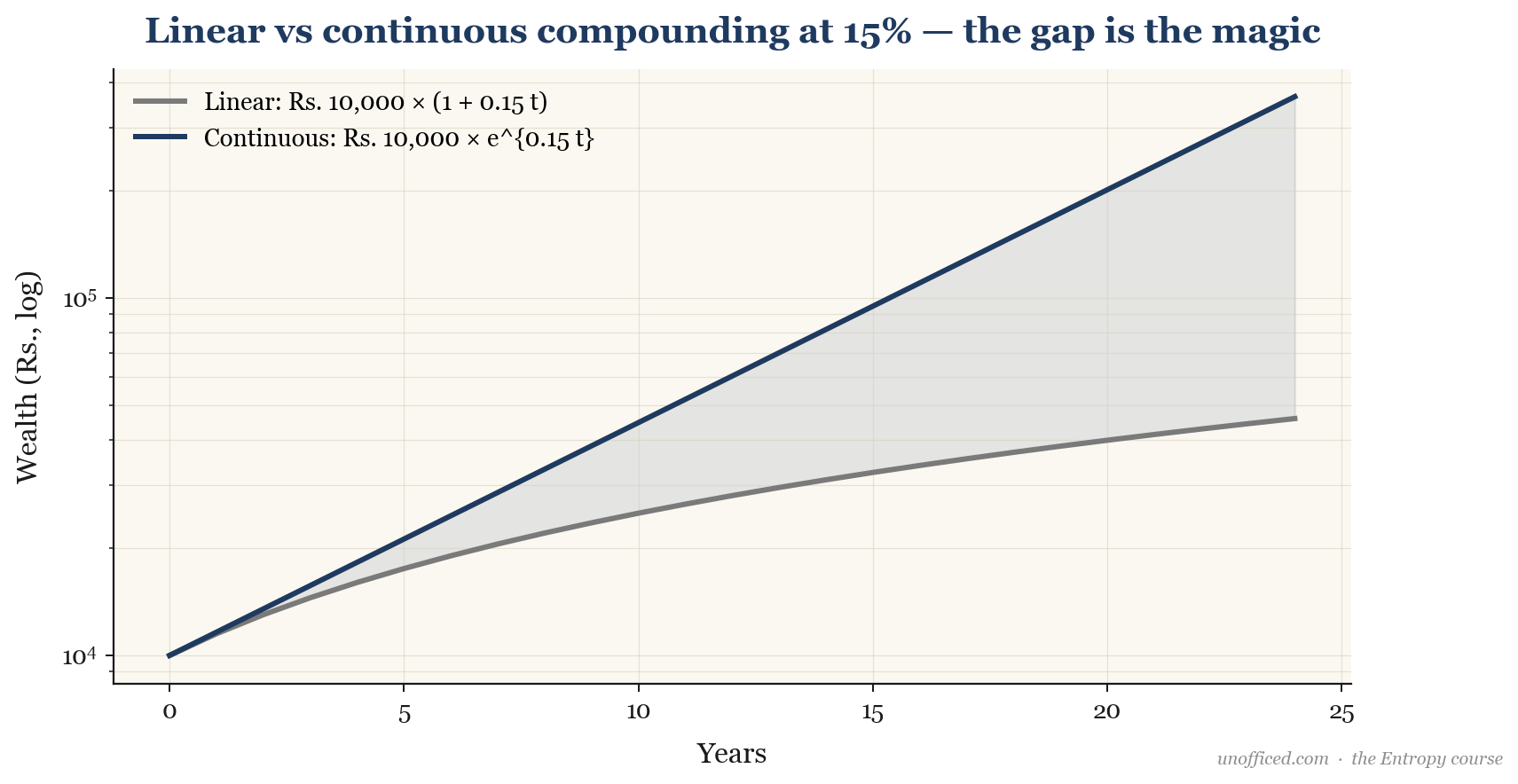
What happens as we increase the compounding frequency, ? Let’s say you invest Rs. 10,000 at a 15% annual interest rate for one year.
| Frequency | n | Calculation | Final Amount (Rs.) |
|---|---|---|---|
| Annual | 1 | 10,000 * (1 + 0.15/1)^1 | 11,500.00 |
| Semi-Annual | 2 | 10,000 * (1 + 0.15/2)^2 | 11,556.25 |
| Quarterly | 4 | 10,000 * (1 + 0.15/4)^4 | 11,586.50 |
| Monthly | 12 | 10,000 * (1 + 0.15/12)^12 | 11,607.55 |
| Daily (Trading Days) | 252 | 10,000 * (1 + 0.15/252)^252 | 11,617.58 |
| Hourly | ~8760 | 10,000 * (1 + 0.15/8760)^8760 | 11,618.31 |
As the compounding frequency increases, the final amount grows, but it appears to be approaching a limit. This demonstrates the move from discrete, linear thinking to a continuous, exponential reality.
The Limit and the Number ‘e’
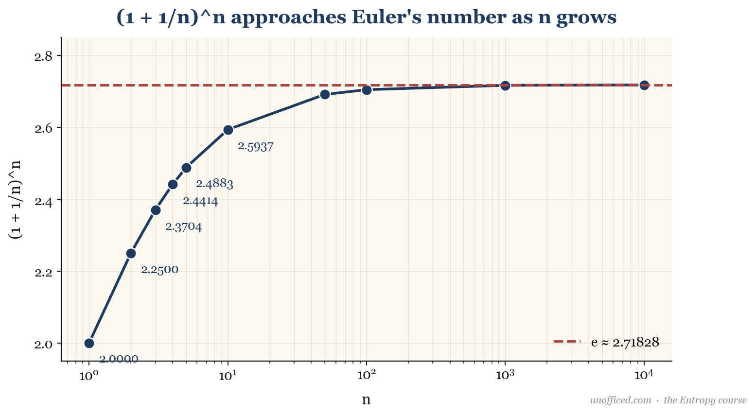
This limit is defined by the mathematical constant (Euler’s number, approx. 2.71828). To see how, we rearrange the formula. Let . As , so does .
The expression inside the brackets is the formal definition of :
This substitution gives us the elegant formula for continuous compounding:
For our example, the value at the limit of continuous compounding would be:
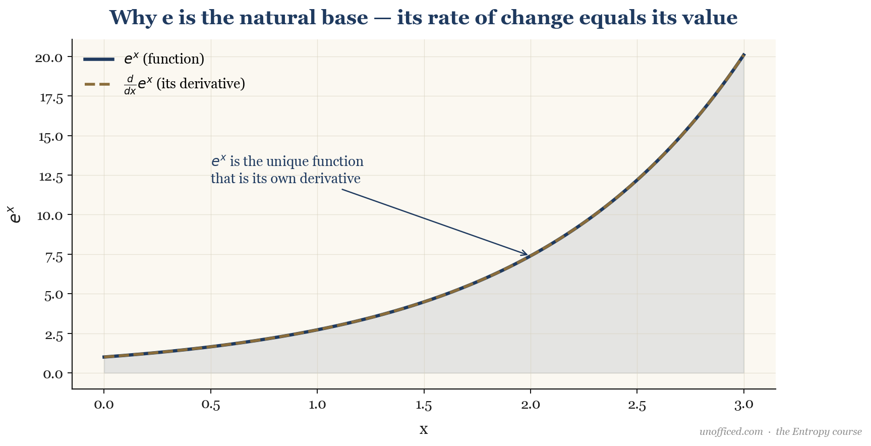
The difference between daily and continuous compounding is often negligible for a single period, but the continuous model is far more mathematically tractable. It’s special because the rate of growth of is equal to its value. This property, where the function is its own derivative, makes it the natural choice for modelling processes where growth is proportional to the current size, like an asset price.
The Rule of 72
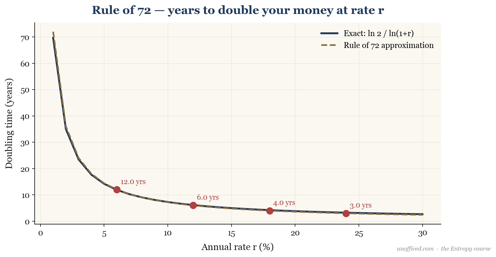
A useful mental shortcut derived from continuous compounding is the “Rule of 72,” which approximates how long it takes for an investment to double. To find the exact doubling time , we solve for in .
To make the math easier for mental calculation, we multiply the numerator and denominator by 100, letting us use as the percentage rate ():
The number 72 is chosen because it’s close to 69.3 and has many divisors, making mental arithmetic simpler.
Here’s how it plays out for different rates:
| Annual Rate (R) | Rule of 72 (Years) | Exact Years (ln(2)/r) |
|---|---|---|
| 5% | 14.4 | 13.86 |
| 10% | 7.2 | 6.93 |
| 15% | 4.8 | 4.62 |
| 20% | 3.6 | 3.47 |
| 25% | 2.88 | 2.77 |
Logarithmic Returns
If continuous compounding describes how prices grow, how do we measure the rate of that growth? We use the natural logarithm, the inverse of the exponential function . By rearranging , we can solve for the single-period continuously compounded return, or log return :
Where is the price at time and is the price at the previous period. Log returns have several properties that make them indispensable for financial analysis.
Key Properties of Log Returns
- Time Additivity: The log return over multiple periods is simply the sum of the log returns for each individual period. The log return from day 0 to day 3 is . This property is invaluable. It is not true for simple returns, making multi-period analysis much cleaner with logs.
- Symmetry: Consider a stock that goes from Rs. 100 to Rs. 120 (+20% simple return) and then back to Rs. 100 (-16.67% simple return). The simple returns are asymmetric and confusing. In log space, the returns are and . They are perfectly symmetric, reflecting the true magnitude of the move.
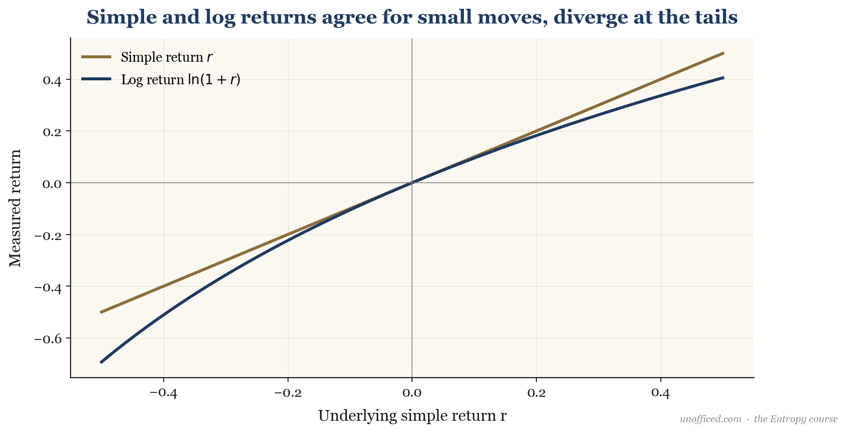
- Approximation for Small Changes: For small values of , the Taylor series expansion holds. This means that for small price changes (e.g., daily returns below 2-3%), the simple return () and log return () are very close in value. They only diverge significantly during large price swings, where the second term becomes meaningful.
Worked Examples
1. Annualising Short-Term Trading Returns
Let’s say a NIFTY options trading portfolio grows from an initial value of Rs. 11,93,403.12 to a final value of Rs. 13,57,361.11 over 40 trading days.
1. Calculate the Simple Return:
2. Calculate the Log Return for the Period:
3. Annualise the Continuously Compounded Rate:
The log return of 12.87% was achieved over 40 trading days. To annualise this, we scale it to a full trading year (approx. 252 days in India).
This tells us the portfolio grew at an annualised, continuously-compounded rate of 81.10%. To state this as an effective annual simple return, we would compute .
2. Calculating CAGR for a Stock Investment
An investor bought shares of Reliance Industries on May 28, 2021, at a price of Rs. 2,080. Five years later, on May 28, 2026, the price is Rs. 3,550.
The simple return over the entire period is . Dividing this by 5 gives a meaningless 14.13% per year. We need the Compound Annual Growth Rate (CAGR).
CAGR is the constant annual rate that would be required to grow the investment from its beginning balance to its ending balance. It’s the geometric mean. We can use log returns to find it easily.
This is the total log return over 5 years. The average annual log return is:
To convert this back to the familiar CAGR, we exponentiate it:
Why Traders and Quants Use Log Returns
Systematic traders, algorithm developers, and quantitative analysts almost exclusively use log returns for modelling, though they use simple returns for accounting.
- Normality Assumption: Many financial models assume returns follow a normal distribution (bell curve). The log returns of assets tend to resemble a normal distribution more closely than simple returns do. This is a critical assumption in many financial models, including the famous Black-Scholes option pricing model, which uses the term to discount future payoffs based on the continuously compounded risk-free rate.
- Stationarity: Price series themselves are non-stationary (their statistical properties like mean and variance change over time). Log return series are often much closer to being stationary, which is a prerequisite for most time-series forecasting models.
- Prevents Negative Prices: When modelling future prices, using log returns ensures the resulting price can never be negative. Since , and the exponential of any real number is positive, the model cannot produce a price below zero. Models based on simple returns can break down and predict absurd negative prices.
- Mathematical Convenience: As shown with time additivity, the mathematical properties of logarithms simplify many calculations required in portfolio optimisation, risk analysis, and derivative pricing.
Further Reading
For those wishing to delve deeper into the mathematics and their application in finance, the following texts are invaluable:
- Options, Futures, and Other Derivatives by John C. Hull. The bible of derivatives pricing, which heavily relies on continuous compounding and lognormal price assumptions.
- An Introduction to the Mathematics of Financial Derivatives by Salih N. Neftci. A more rigorous mathematical treatment of the concepts used in quantitative finance.
- Time Series Analysis by James D. Hamilton. The standard graduate-level textbook for understanding the statistical models applied to return series.
Summary
This lesson provides the conceptual framework for thinking about returns in a way that aligns with financial market dynamics.
- Continuous compounding is the theoretical limit of increasing the frequency of interest payments to infinity, representing exponential growth.
- The formula for continuous growth is , a cornerstone of financial mathematics.
- Logarithmic returns, , are the natural way to measure continuously compounded returns and are the standard for quantitative modelling.
- Log returns are time-additive, making multi-period calculations simple sums.
- For robust modelling, log returns are superior, as they approximate a normal distribution more closely and prevent model-breaking negative prices.
Understanding returns is the first step. Next, we need to describe the behaviour and uncertainty of these returns. This brings us to the concept of a Random Variable.