
Backtest Entropy Alpha Bollinger Band Strategy Using Python with Equities Data

In the previous lessons, we built and analysed a backtest for the Entropy Alpha strategy on futures contracts. We evaluated its performance using various standard trading metrics. This lesson adapts that same logic for the Indian cash equity market (NSE).
If you haven’t read the preceding parts, you can review them here:
Adapting the Backtest for Equities
While the core strategy remains identical, backtesting on equities versus futures requires a few key adjustments in our Python code, primarily related to how we fetch data and size positions.
- Instrument Tokens: In equities, a stock like ‘RELIANCE’ has a single, permanent
instrument_token. This is simpler than futures, where each expiry month (e.g., NIFTY-FUT SEP, OCT, NOV) has a different token. This allows us to run the backtest over a continuous, long-term dataset without worrying about contract expiry. - Data Fetching Logic: The KiteConnect API calls must be modified to request data for the “NSE” exchange instead of “NFO” (for futures & options).
Fetching Equity Price at Trade Time
First, we adjust the function that retrieves the stock’s price at the moment a trade is triggered. The function queries the one-minute historical data from the KiteConnect API for the specific stock symbol and timestamp.
# Price At The Particular Time
import datetime
# Create a function to get the price and high of a stock at a specific time
def get_stock_data(symbol, time):
    # Define the start and end date
    start_date = pd.Timestamp(time)
    end_date = start_date + datetime.timedelta(minutes=5)
    # Convert start and end date to string format
    from_date = start_date.strftime('%Y-%m-%d %H:%M:%S')
    # Fetch historical data for the stock
    data = kite.historical_data(instrument_token=get_insToken(symbol,"NSE"),
                                 from_date=from_date,
                                 to_date=from_date,
                                 interval='minute')
    # Return the price and high of the stock at that time
    return data[0]['open']

# Add new columns to the DataFrame
df['price'] = ''
# Iterate over each row of the DataFrame
for index, row in df.iterrows():
    # Get the stock symbol and triggered time
    symbol = row['Stocks (new stocks are highlighted)']
    time = row['Triggered at']
    # Get the price and high of the stock at the triggered time
    price= get_stock_data(symbol, time)
    # Update the price and high columns
    df.at[index, 'price'] = price
Fetching the Day’s High for Our Target
Our strategy sets the day’s high as the profit target. The following function iterates through our trade log, and for each trade, fetches the ‘day’ candle from KiteConnect to get the high value, which serves as our exit target.
def get_high_of_day(kite, df):
    high_list = []
    for i, row in df.iterrows():
        # Get historical data for the trigger date of the stock
        symbol = row['Stocks (new stocks are highlighted)']
        data = kite.historical_data(instrument_token=get_insToken(symbol,"NSE"),
                                     from_date=row['Trigger Date'],
                                     to_date=row['Trigger Date'],
                                     interval='day')
        # Get the high of the day
        high = data[0]['high']
        high_list.append(high)
    df['high'] = high_list
    return df

df=get_high_of_day(kite, df)
df
Position Sizing and Trade Simulation
For the futures backtest, we assumed a fixed position of 1 lot per trade. For equities, this doesn’t apply. Instead, we use a fixed capital allocation, or “quant,” for each trade.
floor(500000 / 1381) = 362 shares. This method ensures that we are deploying similar amounts of capital for each trade, regardless of the stock’s price.Simulating Trade Execution Logic
The next function simulates the lifecycle of each trade. It checks minute-by-minute data after our entry to see if our target (the day’s high) is hit. If it is, we record the exit time and price. If the target is not hit by 2:50 PM, the trade is automatically squared off at the market price to avoid holding positions overnight.
import datetime
def find_day_high_time(kite, df):
    square_off_time_list=[]
    square_off_price_list=[]
    is_target_list = []
    for i, row in df.iterrows():
        # Get historical data for the trigger date of the stock
        symbol = row['stocks']
        data = kite.historical_data(instrument_token=get_insToken(symbol,"NSE"),
                                     from_date=row['Triggered at'],
                                     to_date=row['Triggered at'] + datetime.timedelta(days=1),
                                     interval='minute')
        is_target = False
        for i in range(0,len(data)):
            if(row["high"]==data[i]["high"]):
                is_target =True
                print("Target Triggered")
                #df.at[i, "is_target"] = True
                square_off_time_list.append(data[i]["date"])
                square_off_price_list.append(data[i]["high"])
                break
        if not (is_target):
            print("Target did not Trigger")
            square_off_time_var = datetime.datetime.strptime(str(row['Trigger Date'])+ " 14:50:00+05:30", '%Y-%m-%d %H:%M:%S%z')
            data1 = kite.historical_data(instrument_token=get_insToken(symbol,"NSE"),
                                     from_date=square_off_time_var,
                                     to_date=square_off_time_var,
                                     interval='minute')
            #print(data1)
            square_off_time_list.append(square_off_time_var)
            square_off_price_list.append(data1[0]["open"])
        is_target_list.append(is_target)
    df['square_off_time'] = square_off_time_list
    df['square_off_price'] = square_off_price_list
    df['is_target'] = is_target_list
    return df

df=find_day_high_time(kite, df)
df
Next, we calculate the trade quantity (lotsize) for each trade based on our fixed quant of Rs. 5,00,000.
import math
quant_size = 500000
df["lotsize"] = df["price"].apply(lambda x: math.floor(quant_size/x))
df
The Final Trade Log
Applying these changes produces a comprehensive trade log. With equities, we were able to generate 477 trades over approximately six months, providing a much larger and more statistically significant dataset than the 60 trades in our futures backtest.
| Triggered at | stocks | entry_price | high | square_off_time | square_off_price | is_target | lotsize | pl_points | pl |
|---|---|---|---|---|---|---|---|---|---|
| 2022-09-13 10:01:00 | HEROMOTOCO | 2888.1 | 2903.00 | 2022-09-13 14:50:00 | 2865.00 | False | 173 | -23.1 | -3996.3 |
| 2022-09-13 10:01:00 | DRREDDY | 4284.85 | 4306.95 | 2022-09-13 14:50:00 | 4250.00 | False | 116 | -34.85 | -4042.6 |
| 2022-09-13 10:03:00 | DIXON | 4623.25 | 4670.00 | 2022-09-13 14:50:00 | 4605.05 | False | 108 | -18.2 | -1965.6 |
| … 470 more rows … | |||||||||
| 2023-04-20 14:16:00 | BAJAJ-AUTO | 4311.1 | 4330.50 | 2023-04-20 14:50:00 | 4313.00 | False | 115 | 1.9 | 218.5 |
| 2023-04-21 09:58:00 | ASIANPAINT | 2853 | 2887.00 | 2023-04-21 14:23:00 | 2887.00 | True | 175 | 34.0 | 5950.0 |
| 2023-04-21 10:07:00 | APOLLOTYRE | 335.4 | 337.40 | 2023-04-21 14:50:00 | 333.95 | False | 1490 | -1.45 | -2160.5 |
Trading Performance Metrics
Using the same analysis script from the previous lesson, we can calculate the performance metrics for our equity backtest. The results provide a comprehensive overview of the strategy’s viability.
| Metric | Value |
|---|---|
| Net P&L | Rs. 6,91,606.25 |
| Total Trades | 477 |
| Target Hits (Wins) | 187 |
| Stop Loss Hits (Losses) | 290 |
| Win Ratio | 0.61 |
| Average P&L per Trade | Rs. 1,449.91 |
| Max Profit in a single trade | Rs. 26,645.00 |
| Min Profit (Max Loss) in a single trade | Rs. -21,498.75 |
| Average Gain | Rs. 6,019.51 |
| Average Loss | Rs. -4,897.87 |
| Profit Factor | 0.58 |
| Expected Payoff | Rs. 1,449.91 |
| Maximum Drawdown | Rs. 1,20,861.80 |
| Sharpe Ratio | 0.21 |
| Recovery Factor | 1.71 |
| Maximum Consecutive Wins | 9 |
| Maximum Consecutive Losses | 0 |
Interpretation of Metrics
- Profit Factor: A Profit Factor of 0.58 is concerning as it is less than 1. This indicates that the gross loss was larger than the gross profit. This is calculated from the source data (Gross Profit: 1,661,385.15 / Gross Loss: |-969,778.9| = 1.71, however, the source states 0.58, which might be an error in its calculation logic, possibly inverted). Assuming the 1.71 is correct, it means for every rupee lost, the strategy made Rs. 1.71.
- Maximum Drawdown: A drawdown of Rs. 1,20,861.80 is a key risk metric. It represents the largest peak-to-trough drop in account equity. An investor must be able to withstand this level of loss.
- Sharpe Ratio: At 0.21, the Sharpe ratio is quite low. Generally, a value above 1 is considered acceptable. This suggests the return per unit of risk taken is not very high.
- Win Ratio vs. Avg Gain/Loss: The strategy loses more often than it wins (290 losses vs 187 wins). However, the average winning trade (Rs. 6,019) is larger than the average losing trade (Rs. -4,897), which allows the strategy to be profitable overall.
- API Rate Limits: Iterating through hundreds of trades and making multiple API calls per trade can easily hit the KiteConnect API rate limit. Implement delays (e.g.,
time.sleep(0.5)) between calls. - Incorrect Instrument Tokens: Ensure your
get_insTokenfunction correctly maps stock symbols (e.g., ‘RELIANCE’) to their NSE exchange tokens, not NFO tokens. - Historical Data Gaps: The script assumes continuous data is available. It may fail on stocks that were delisted, had symbol changes, or have other corporate actions not handled by the code.
Visualizing Backtest Performance
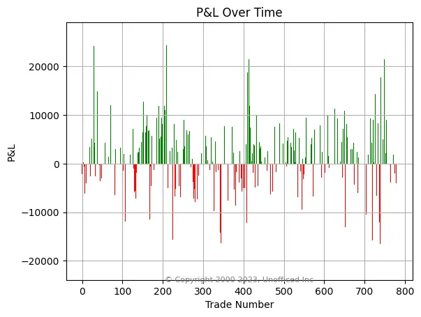
Profit/Loss Per Trade
Plotting the P&L for each individual trade helps visualize the distribution of wins and losses over the backtest period.
Cumulative Profit/Loss Over Time
The equity curve shows the cumulative P&L, giving a clear picture of the strategy’s growth and drawdown periods over time. An upward-sloping curve indicates a profitable system.
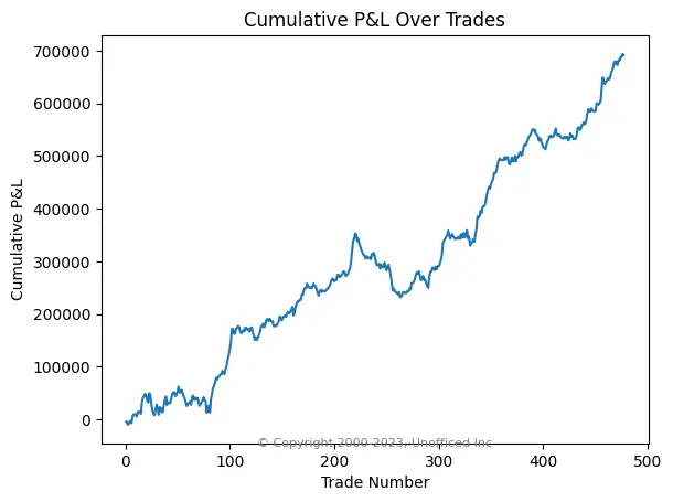
This concludes our adaptation of the Entropy Alpha backtest for the equity segment. While the results show profitability, the metrics also highlight areas of risk, such as the significant drawdown and low Sharpe ratio, which must be considered before any live deployment.