Navigating the Randomness: How the Wiener Process Alters Sharpe Ratios

In algorithmic trading, it’s important to use metrics to evaluate how effective an investment strategy is. One such metric is the Sharpe Ratio, which measures the return of an investment compared to its risk.
This article looks at how the Wiener Process affects the Sharpe Ratio for the stock of SBIN. By simulating stock prices with the Geometric Brownian Motion, we can see how the actual Sharpe Ratios compare to what we would theoretically expect. This highlights the role of randomness in financial analysis and the need to be cautious when making decisions based on these metrics.
Calculating Sharpe Ratios on GBM Simulations
In the last chapter, We have learned How to Simulate Geometric Brownian Motion in a Stock , Now, How about We compute the Sharpe Ratio for the SBIN stock for all these various paths? The formula for the Sharpe Ratio is:
$$\text{Sharpe Ratio} = \frac{R_p – R_f}{\sigma_p}$$
Where:
- \(R_p\) is the mean return of the investment
- \(R_f\) is the risk-free rate
- \(\sigma_p\) is the standard deviation of the investment (or portfolio)
For the sake of this simulation, we’ll assume a risk-free rate (typically, this could be the return of a 10-year government bond or another similar secure investment) as 10%.
Here’s the simulation, calculation, and interpretation:
					import numpy as np
from datetime import datetime, timedelta

def simulate_gbm(S0, mu, sigma, dt, num_days, num_simulations):
    stock_price_paths = np.zeros((num_days, num_simulations))
    stock_price_paths[0] = S0

    for t in range(1, num_days):
        rand_nums = np.random.randn(num_simulations)
        stock_price_paths[t] = stock_price_paths[t - 1] * np.exp((mu - 0.5 * sigma**2) * dt + sigma * np.sqrt(dt) * rand_nums)

    return stock_price_paths

# Fetching the drift and volatility from previously defined functions
end_date = datetime.today().strftime('%d-%m-%Y')
start_date = (datetime.today() - timedelta(days=100)).strftime('%d-%m-%Y')
symbol = "SBIN"
series = "EQ"

daily_drift = get_daily_drift(symbol, series, start_date, end_date)
daily_volatility = get_daily_volatility(symbol, series, start_date, end_date)

# Parameters for the simulation
S0 = equity_history(symbol, series, start_date, end_date)['CH_CLOSING_PRICE'].iloc[0]
mu = daily_drift
sigma = daily_volatility
dt = 1/252
num_days = 100
num_simulations = 10000

stock_price_paths = simulate_gbm(S0, mu, sigma, dt, num_days, num_simulations)

# Calculating the Sharpe Ratio
Rf = 0.1 / 252  # Assuming a 10% annual risk-free rate, which is then converted to a daily rate
Rp = np.mean((stock_price_paths[-1] - stock_price_paths[0]) / stock_price_paths[0])
sharpe_ratio = (Rp - Rf) / sigma

print(f"Calculated Sharpe Ratio for SBIN: {sharpe_ratio}")
Output:
Calculated Sharpe Ratio for SBIN: -0.022685478221275538
Plotting Varations of Sharpe Ratio
The provided code simulates the stock price paths of SBIN over 100 days based on the Geometric Brownian Motion and then calculates the Sharpe Ratio using the risk-free rate and standard deviation.
Make sure to adjust the risk-free rate (\(R_f\)) according to current market conditions or any other rate you deem appropriate.
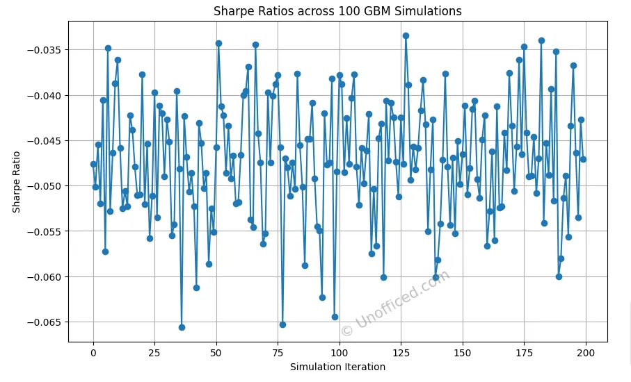
Each time you run the simulation, you’ll get a different Sharpe Ratio due to the random component (the Wiener process) in the Geometric Brownian Motion. Let’s run the simulation 200 times, storing the calculated Sharpe Ratio in each iteration, and then plot these values.
# Simulation parameters
S0 = 552.4  # Assuming this as the current price, you may want to update it
dt = 1/252
num_days = 100
num_simulations = 10000
Rf = 0.1 / 252

# Run the GBM simulation 200 times and store Sharpe Ratios
sharpe_ratios = []
for _ in range(200):
    stock_price_paths = simulate_gbm(S0, daily_drift, daily_volatility, dt, num_days, num_simulations)
    Rp = np.mean((stock_price_paths[-1] - stock_price_paths[0]) / stock_price_paths[0])
    sharpe_ratio = (Rp - Rf) / daily_volatility
    sharpe_ratios.append(sharpe_ratio)

# Plot the Sharpe Ratios
plt.figure(figsize=(10, 6))
plt.plot(sharpe_ratios, marker='o')
plt.xlabel('Simulation Iteration')
plt.ylabel('Sharpe Ratio')
plt.title('Sharpe Ratios across 100 GBM Simulations')
plt.grid(True)
plt.annotate("© Unofficed.com",
             xy=(0.5, 0.01),  # Change the placement if needed
             xycoords="axes fraction",
             fontsize=15,
             alpha=0.5,
             color="gray",  # Change to a contrasting color
             rotation=30)
plt.show()
Output:
Interpreting the Results:
The reason we perform this simulation multiple times is to understand the potential variability in stock price paths based on the random component (the Wiener process).
From the example given, Let’s calculate the average measured Sharpe ratio –
					# Calculate the average Sharpe ratio from the simulated values
average_measured_sharpe_ratio = np.mean(sharpe_ratios)
print(f"Average measured Sharpe ratio is: {average_measured_sharpe_ratio}")
Output:
Average measured Sharpe ratio is: -0.04721741885398455
Let’s calculate the theoretical value using the Sharpe Ratio function –
					# Calculate the theoretical Sharpe ratio for SBIN
sbin_theoretical_sharpe_ratio = sharpe_ratio("SBIN", "EQ", 10, start_date, end_date)
print(f"Theoretical Sharpe Ratio for SBIN: {sbin_theoretical_sharpe_ratio}")
Output:
Theoretical Sharpe Ratio for SBIN: -49.85863670573091
This suggests that the noise (random fluctuations) introduced by the Wiener process impacts the Sharpe ratio calculations. The Sharpe ratio, when computed on these simulated returns, can vary from its expected theoretical value due to this randomness.