Buy on RSI Strategy Coding in Python using Zerodha

This is a programming lesson. So there will be very less amount of explanation and more code. If you’re stuck somewhere, feel free to comment.
Objective
Execute a buy order for Sun Pharma stock based on specific conditions –
- Trigger the buy order when the Relative Strength Index (RSI) surpasses 30.
- Additionally, require that the current high of a candlestick is higher than the previous high of the candlestick.
If these conditions are satisfied, then place a limit order for Sun Pharma stock.
Note – The structure of historical data and live data from Zerodha is identical. During the development and testing of functions, it’s not feasible to wait for days or months to validate their performance using live data.
To address this, we’ll initially test and validate our functions using historical data. Once we have confirmed that the functions generate accurate signals and execute trades correctly with historical data, we can seamlessly transition to using live data for real-time trading.
Python Code
					def get_historical_data(kite, instrument_token, start_date, end_date, interval):
    return kite.historical_data(instrument_token, start_date, end_date, interval, 0)

def calculate_rsi(za):
    rsi_period = 14
    chg = za["close"].diff(1)
    gain = chg.mask(chg < 0, 0)
    loss = chg.mask(chg > 0, 0)
    avg_gain = gain.ewm(com=rsi_period - 1, min_periods=rsi_period).mean()
    avg_loss = loss.ewm(com=rsi_period - 1, min_periods=rsi_period).mean()
    rs = abs(avg_gain / avg_loss)
    rsi = 100 - (100 / (1 + rs))
    za['rsi'] = rsi
    return za.iloc[-1, 6]

def place_order(kite, symbol, quantity, price, transaction_type):
    kite.place_order(
        variety="regular",
        tradingsymbol=symbol,
        quantity=quantity,
        exchange='NSE',
        order_type='LIMIT',
        price=price,
        transaction_type=transaction_type,
        product='CNC'
    )
    print("One order placed")

def livedata():
    while True:
        km = datetime.datetime.now().minute
        ks = datetime.datetime.now().second
        if km % 1 == 0 and ks == 1:
            historical_data = get_historical_data(kite, 857857, "2019-01-05", "2019-06-02", "minute")
            za = pd.DataFrame(historical_data)
            rsi_value = calculate_rsi(za)

            if rsi_value > 30 and za.iloc[-2, 2] > za.iloc[-1, 2]:
                place_order(kite, 'SUNPHARMA', 1, 453, 'BUY')
                break
            else:
                pass
            time.sleep(60)

livedata()
Output –
File ~/apps/zerodha/../kiteconnect/connect.py:671, in KiteConnect._request(self, route, method, parameters)
    669         # native Kite errors
    670         exp = getattr(ex, data["error_type"], ex.GeneralException)
--> 671         raise exp(data["message"], code=r.status_code)
    673     return data["data"]
    674 elif "csv" in r.headers["content-type"]:

InputException: interval exceeds max limit: 60 days
The error message indicates that the specified time interval for data retrieval exceeds the maximum limit, which is set to 60 days. This means you cannot retrieve data for a period longer than 60 days using the given interval.
So, Let’s modify the historical_data request to fetch data for today and the past 50 days.
					start_date = (datetime.date.today() - datetime.timedelta(days=50)).strftime("%Y-%m-%d")
end_date = datetime.date.today().strftime("%Y-%m-%d")

def livedata():
    while True:
        km = datetime.datetime.now().minute
        ks = datetime.datetime.now().second
        if km % 1 == 0 and ks == 1:
            historical_data = get_historical_data(kite, 857857, start_date, end_date, "minute")
            za = pd.DataFrame(historical_data)
            rsi_value = calculate_rsi(za)

            if rsi_value > 30 and za.iloc[-2, 2] > za.iloc[-1, 2]:
                print("RSI Value is " +str(rsi_value))
                place_order(kite, 'SUNPHARMA', 1, 453, 'BUY')
                break
            else:
                pass
            time.sleep(60)

livedata()
Output –
					RSI Value is 35.53216733131616
One order placed
Plot RSI Graph Part I
					import matplotlib.pyplot as plt

historical_data = get_historical_data(kite, 857857, start_date, end_date, "minute")
za = pd.DataFrame(historical_data)

rsi_values = []  # List to store RSI values

for i in range(len(za)):
    # Create a DataFrame containing a single row from 'za'
    single_row = pd.DataFrame(za.iloc[i]).T
    rsi_value = calculate_rsi(single_row)
    rsi_values.append(rsi_value)

plt.figure(figsize=(12, 6))
plt.plot(za["date"], rsi_values, label="RSI", color='blue')
plt.axhline(y=30, color='red', linestyle='--', label="RSI 30")
plt.axhline(y=70, color='green', linestyle='--', label="RSI 70")
plt.title("RSI Between {} and {}".format(start_date, end_date))
plt.xlabel("Date")
plt.ylabel("RSI Value")
plt.legend()
plt.grid(True)
plt.show()
Output –
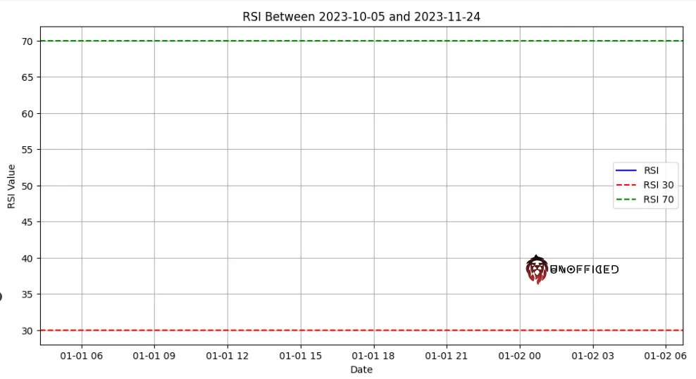
So, Let’s debug –
print(za)
Output –
					date	open	high	low	close	volume
0	2023-10-05 09:15:00+05:30	1124.65	1128.65	1122.80	1124.45	19041
1	2023-10-05 09:16:00+05:30	1125.20	1126.50	1125.05	1126.50	7274
2	2023-10-05 09:17:00+05:30	1126.10	1127.45	1125.50	1127.00	6414
3	2023-10-05 09:18:00+05:30	1127.00	1128.05	1125.85	1125.85	3172
4	2023-10-05 09:19:00+05:30	1125.85	1126.35	1125.00	1125.65	5333
...	...	...	...	...	...	...
13051	2023-11-24 13:16:00+05:30	1194.40	1194.50	1193.35	1193.95	2385
13052	2023-11-24 13:17:00+05:30	1193.95	1194.45	1193.55	1193.70	1695
13053	2023-11-24 13:18:00+05:30	1194.35	1195.00	1193.65	1195.00	5209
13054	2023-11-24 13:19:00+05:30	1195.00	1195.30	1194.05	1194.75	3679
13055	2023-11-24 13:20:00+05:30	1194.75	1194.75	1194.10	1194.10	84
13056 rows × 6 columns
print(rsi_values)
Output –
					[nan,
 nan,
 nan,
 nan,
 nan,
 nan,
 nan,
 nan,
 nan,
 nan,
 nan,
 nan,
 ...
 ...]
To calculate the Relative Strength Index (RSI) for a specific day, you require data from the previous 14 days. Therefore, you should create a separate function to calculate the RSI for each day, excluding the first 14 days where RSI cannot be calculated due to insufficient historical data. This function will compute the RSI values and return a list of RSI values for the remaining days in your dataset.
Here’s an example of how to create such a function and use it in your code.
					def calculate_rsi_list(df):
    rsi_period = 14
    rsi_values = []

    for i in range(len(df)):
        if i < rsi_period:
            rsi_values.append(None)  # Cannot calculate RSI for the first 14 days
        else:
            chg = df["close"].diff(1)
            gain = chg.where(chg > 0, 0)
            loss = -chg.where(chg < 0, 0)
            avg_gain = gain.iloc[i - rsi_period + 1:i + 1].mean()
            avg_loss = loss.iloc[i - rsi_period + 1:i + 1].mean()
            if avg_loss == 0:
                rsi = 100
            else:
                rs = avg_gain / avg_loss
                rsi = 100 - (100 / (1 + rs))
            rsi_values.append(rsi)

    return rsi_values

rsi_values = calculate_rsi_list(za)
print(rsi_values)
Output –
[None, None, None, None, None, None, None, None, None, None, None, None, None, None, 39.730639730639666, 30.078124999999943, 26.377952755905184, 27.459016393442283, 32.9457364341083, 39.50177935943041, 41.240875912409294, 43.840579710144745, 44.322344322344435, 43.999999999999666, 44.322344322344435, 38.43416370106739, 38.848920863308756, 21.513944223108012, 35.08771929824533, 38.84297520661151, 39.49579831932781, 41.409691629956676, 37.850467289719845, 37.26415094339563, 35.648148148146845, 39.0350877192979, 47.39130434782545, 56.476683937824085, 56.92307692307779, 55.778894472362374, 60.655737704918444, 71.33757961783407, 67.85714285714286, 61.83206106870202, 63.77952755905532, 71.05263157894643, 61.67664670658586, 55.24475524475518, 60.81081081081126, 52.63157894736933, 44.73684210526421, 50.0, 48.0314960629921, ...]
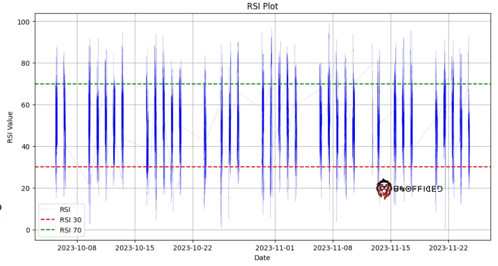
Plot RSI Graph Part II
So, Let’s plot this RSI data against dates.
					import matplotlib.pyplot as plt

# Assuming you have already calculated the rsi_values using calculate_rsi_list

plt.figure(figsize=(12, 6))
plt.plot(za["date"],rsi_values, label="RSI", color='blue', linewidth=0.1)
plt.axhline(y=30, color='red', linestyle='--', label="RSI 30")
plt.axhline(y=70, color='green', linestyle='--', label="RSI 70")
plt.title("RSI Plot")
plt.xlabel("Date")
plt.ylabel("RSI Value")
plt.legend()
plt.grid(True)
plt.show()
Output –